arX

iv:0

907.

0116

v2 [

mat

h.D

S] 1

7 Se

p 20

09

An entire transcendental family with a persistent

Siegel disc

Ruben Berenguel∗, Nuria Fagella†

June 11, 2013

Abstract

We study the class of entire transcendental maps of finite order withone critical point and one asymptotic value, which has exactly one finitepre-image, and having a persistent Siegel disc. After normalisation this isa one parameter family fa with a ∈ C∗ which includes the semi-standardmap λzez at a = 1, approaches the exponential map when a → 0 anda quadratic polynomial when a → ∞. We investigate the stable compo-nents of the parameter plane (capture components and semi-hyperboliccomponents) and also some topological properties of the Siegel disc interms of the parameter.

1 Introduction

Given a holomorphic endomorphism f : S → S on a Riemann surface S weconsider the dynamical system generated by the iterates of f , denoted by fn =

fn· · · f . The orbit of an initial condition z0 ∈ S is the sequence O+(z0) =

fn(z0)n∈N and we are interested in classifying the initial conditions in thephase space or dynamical plane S, according to the asymptotic behaviour oftheir orbits when n tends to infinity.

There is a dynamically natural partition of the phase space S into the Fatouset F (f) (open) where the iterates of f form a normal family and the Julia setJ (f) = S\F (f) which is its complement (closed).

If S = C = C ∪ ∞ then f is a rational map. If S = C and f does notextend to the point at infinity, then f is an entire transcendental map, that is,infinity is an essential singularity. Entire transcendental functions present manydifferences with respect to rational maps.

One of them concerns the singularities of the inverse function. For a rationalmap, all branches of the inverse function are well defined except at a finitenumber of points called the critical values, points w = f(c) where f ′(c) = 0.The point c is then called a critical point. If f is an entire transcendental

∗Email: ruben@maia.ub.es†Email: fagella@maia.ub.es

1

map, there is another possible obstruction for a branch of the inverse to be welldefined, namely its asymptotic values. A point v ∈ C is called an asymptoticvalue if there exists a path γ(t) → ∞ when t → ∞, such that f(γ(t)) → v ast→ ∞. An example is v = 0 for f(z) = ez, where γ(t) can be chosen to be thenegative real axis.

In any case, the set of singularities of the inverse function, also called singu-lar values, plays a very important role in the theory of iteration of holomorphicfunctions. This statement is motivated by the non-trivial fact that most con-nected components of the Fatou set (or stable set) are somehow associated to asingular value. Therefore, knowing the behaviour of the singular orbits providesinformation about the nature of the stable orbits in the phase space.

The dynamics of rational maps are fairly well understood, given the fact thatthey possess a finite number of critical points and hence of singular values. Thismotivated the definition and study of special classes of entire transcendentalfunctions like, for example, the class S of functions of finite type which arethose with a finite number of singular values. A larger class is B the classof functions with a bounded set of singularities. These functions share manyproperties with rational maps, one of the most important is the fact that everyconnected component of the Fatou set is eventually periodic (see e.g. [7] or[11]). There is a classification of all possible periodic connected components ofthe Fatou set for rational maps or for entire transcendental maps in class S.Such a component can only be part of a cycle of rotation domains (Siegel discs)or part of the basin of attraction of an attracting, super-attracting or parabolicperiodic orbit.

We are specially interested in the case of rotation domains. We say that ∆is an invariant Siegel disc if there exists a conformal isomorphism ϕ : ∆ → D

which conjugates f to Rθ(z) = e2πiθz (and ϕ can not be extended further),with θ ∈ R \ Q ∩ (0, 1) called the rotation number of ∆. Therefore a Siegeldisc is foliated by invariant closed simple curves, where orbits are dense. Theexistence of such Fatou components was first settled by Siegel [24] who showedthat if z0 is a fixed point of multiplier ρ = f ′(z0) = e2πiθ and θ satisfies aDiophantine condition, then z0 is analytically linearisable in a neighbourhoodor, equivalently, z0 is the centre of a Siegel disc. The Diophantine conditionwas relaxed later by Brjuno and Russman (for an account of these proofs seee.g. [17]), who showed that the same is true if θ belonged to the set of Brjunonumbers B. The relation of Siegel discs with singular orbits is as follows. Clearly∆ cannot contain critical points since the map is univalent in the disc. Instead,the boundary of ∆ must be contained in the post-critical set ∪c∈Sing(f−1)O+(c)i.e., the accumulation set of all singular orbits. In fact something stronger istrue, namely that ∂∆ is contained in the accumulation set of the orbit of atleast one singular value (see [15]).

Our goal in this paper is to describe the dynamics of the one parameterfamily of entire transcendental maps

fa(z) = λa(ez/a(z + 1 − a) − 1 + a),

where a ∈ C \ 0 = C∗ and λ = e2πiθ with θ being a fixed irrational Brjuno

2

number. Observe that 0 is a fixed point of multiplier λ and therefore, for allvalues of the parameter a, there is a persistent Siegel disc ∆a around z = 0.The functions fa have two singular values: the image of the only critical pointw = −1 and an asymptotic value at va = λa(a− 1) which has one and only onefinite pre-image at the point pa = a− 1.

The motivation for studying this family of maps is manifold. On one handthis is the simplest family of entire transcendental maps having one simplecritical point and one asymptotic value with a finite pre-image (see Theorem3.18 for the actual characterisation of fa). The persistent Siegel disc makesit into a one-parameter family, since one of the two singular orbits must beaccumulating on the boundary of ∆a. We will see that the situation is verydifferent, depending on which of the two singular values is doing that. Therefore,these maps could be viewed as the transcendental version of cubic polynomialswith a persistent invariant Siegel disc, studied by Zakeri in [28]. In our case,many new phenomena are possible with respect to the cubic situation, likeunbounded Siegel discs for example; but still the two parameter planes sharemany features like the existence of capture components or semi-hyperbolic ones.

There is a second motivation for studying the maps fa, namely that thisone parameter family includes in some sense three emblematic examples. Fora = 1 we have the function f1(z) = λzez, for large values of a we will seethat fa is polynomial-like of degree 2 in a neighbourhood of the origin (seeTheorem 3.19); finally when a → 0, the dynamics of fa are approaching thoseof the exponential map u 7→ λ(eu − 1), as it can be seen changing variables tou = z/a. Thus the parameter plane of fa can be thought of as containing the

polynomial λ(z + z2

2 ) at infinity, its transcendental analogue f1 at a = 1, andthe exponential map at a = 0. The maps z 7→ λzez have been widely studied(see [10] and [8]), among other reasons, because they share many propertieswith quadratic polynomials: in particular it is known that when θ is of constanttype, the boundary of the Siegel disc is a quasi-circle that contains the criticalpoint. It is not known however whether there exist values of θ for which theSiegel disc of f1 is unbounded. In the long term we hope that this family facan throw some light into this and other problems about f1.

For the maps at hand we prove the following.

Theorem A. a) There exists R,M > 0 such that if θ is of constant type and|a| > M then the boundary of ∆a is a quasi-circle which contains the criticalpoint. Moreover ∆a ⊂ D(0, R).

b) If θ is Diophantine and the orbit of c = −1 belongs to a periodic basin oris eventually captured by the Siegel disc, then either the Siegel disc ∆a isunbounded or its boundary is an indecomposable continuum.

c) If θ is Diophantine and fna (−1)n→∞−→ ∞ the Siegel disc ∆a is unbounded,

and the boundary contains the asymptotic value.

Part a) follows from Theorem 3.19 (see Corollary 1 below it). The remainingparts (Theorem 3.20) are based on Herman’s proof [12] of the fact that Siegel

3

discs of the exponential map are unbounded, if the rotation number is Diophan-tine, although in this case there are some extra difficulties given by the freecritical point and the finite pre-image of the asymptotic value.

In this paper we are also interested in studying the parameter plane of fa,which is C∗, and in particular the connected components of its stable set, i.e., theparameter values for which the iterates of both singular values form a normalfamily in some neighbourhood. We denote this set as S (not to be confusedwith the class of finite type functions). These connected components are eithercapture components, where an iterate of the free singular value falls into theSiegel disc; or semi-hyperbolic, when there exists an attracting periodic orbit(which must then attract the free singular value); otherwise they are calledqueer.

The following theorem summarises the properties of semi-hyperbolic com-ponents, and is proved in Section 4 (see Proposition 4, Theorems 4.22, 4.23and Proposition 5 therein). By a component of a set we mean a connectedcomponent.

Theorem B. Define

Hc = a ∈ C|O+(−1) is attracted to an attracting periodic orbit,

Hv = a ∈ C|O+(va) is attracted to an attracting periodic orbit.

a) Every component of Hv ∪Hc is simply connected.

b) If W is a component of Hv then W is unbounded and the multiplier mapχ : W → D∗ is the universal covering map.

c) There is one component Hv1 of Hv for which O+(va) tends to an attracting

fixed point. Hv1 contains the segment [r,∞) for r large enough.

d) If W is a component of Hc, then W is bounded and the multiplier mapχ : W → D is a conformal isomorphism.

Indeed, when the critical point is attracted by a cycle, we naturally see copiesof the Mandelbrot set in parameter space. Instead, when it is the asymptoticvalue that acts in a hyperbolic fashion, we find unbounded exponential-likecomponents, which can be parametrised using quasi-conformal surgery.

A dichotomy also occurs with capture components. Numerically we canobserve copies of quadratic Siegel discs in parameter space, which correspondto components for which the asymptotic value is being captured. There is in facta main capture component Cv0 , the one containing a = 1 (see Figure 1), whichcorresponds to parameters for which the asymptotic value va, belongs itself tothe Siegel disc. This is possible because of the existence of a finite pre-imageof va. The centre of Cv0 is the semi-standard map f1(z) = λzez, for which zeroitself is the asymptotic value.

The properties we show for capture components are summarised in the fol-lowing theorem (see Section 5: Theorem 5.24 and Proposition 7).

4

Theorem C. Let us define

Cc = a ∈ C|fna (−1) ∈ ∆a for some n ≥ 1,

Cv = a ∈ C|fna (va) ∈ ∆a for some n ≥ 0.

Then

a) Cc and Cv are open sets.

b) Every component W of Cc ∪Cv is simply connected.

c) Every component W of Cc is bounded.

d) There is only one component of Cv0 = a ∈ C|va ∈ ∆a and it is bounded.

Numerical experiments show that if θ is of constant type, the boundary ofCv0 is a Jordan curve, corresponding to those parameter values for which bothsingular values lie on the boundary of the Siegel disc (see Figure 1). This is truefor the slice of cubic polynomials having a Siegel disc of rotation number θ, asshown by Zakeri in [28], but his techniques do not apply to this transcendentalcase.

H2

H2

H1

0 1 11

Figure 1: Left: Simple escape time plot of the parameter plane. Light grey:asymptotic orbit escapes, dark grey critical orbit escapes, white neither escapes.Regions labelled H1 and H2 correspond to parameters for which the asymptoticvalue is attracted to an attracting cycle. Right: The same plot, using a differentalgorithm which emphasises the capture components. Upper left: (−2, 2), Lowerright: (4,−4).

As we already mentioned, we are also interested in parameter values forwhich fa is Julia stable, i.e. where both families of iterates fna (−1)n∈N andfna (va)n∈N are normal in a neighbourhood of a (see Section 6). We first showthat any parameter in a capture component or a semi-hyperbolic component isJ -stable.

5

Proposition 1. If a ∈ H ∪ C then fa is J -stable, where H = Hc ∪ Hv andC = Cc ∪ Cv.

By using holomorphic motions and the proposition above, it is enough tohave certain properties for one parameter value a0, to be able to “extend” themto all parameters belonging to the same stable component. More precisely weobtain the following corollaries (see Proposition 8 and Corollary 3).

Proposition 2. a) If θ is of constant type and a ∈ Cv0 (i.e. the asymptoticvalue lies inside the Siegel disc) then ∂∆a is a quasi-circle that contains thecritical point.

b) Let W ⊂ Hv ∪ Cv be a component intersecting |z| > M where M is as inTheorem A. Then,

i) if θ is of constant type, for all a ∈W the boundary ∂∆a is a quasi-circlecontaining the critical point.

ii) There exist values of θ ∈ R\Q ∩ (0, 1) such that if a component W ⊂Cv ∪Hv intersects |z| > M, then for all a ∈ W , the boundary of ∆a

is a quasi-circle not containing the critical point.

The paper is organised as follows. Section 2 contains statements and refer-ences of some of the results used throughout the paper. Section 3 contains thecharacterisation of the family fa, together with descriptions and images of thepossible scenarios in dynamical plane. It also contains the proof of TheoremA. Section 4 deals with semi-hyperbolic components and contains the proof ofTheorem B, split in several parts, and not necessarily in order. In the samefashion, capture components and Theorem C are treated in Section 5. FinallySection 6 investigates Julia stability and contains the proofs of Propositions Dand E.

2 Preliminary results

In this section we state results and definitions which will be useful in the sectionsto follow.

2.1 Quasi-conformal mappings and holomorphic motions

First we introduce the concept of quasi-conformal mapping. Quasi-conformalmappings are a very useful tool in complex dynamical systems as they provide abridge between a geometric construction for a system and its analytic informa-tion. They are also a fundamental pillar for the framework of quasi-conformalsurgery, the other one being the measurable Riemann mapping theorem. Forthe groundwork on quasi-conformal mappings see for example [1], and for anexhaustive account on quasi-conformal surgery, see [4].

6

Definition 1. Let µ : U ⊆ C → C be a measurable function. Then it is a k-Beltrami form (or Beltrami coefficient, or complex dilatation) of U if ‖µ(z)‖∞ ≤k < 1.

Definition 2. Let f : U ⊆ C → V ⊆ C be a homeomorphism. We call itk-quasi-conformal if locally it has distributional derivatives in L2 and

µf (z) =∂f∂z (z)∂f∂z (z)

(1)

is a k-Beltrami coefficient. Then µf is called the complex dilatation of f(z) (orthe Beltrami coefficient of f(z)).

Given f(z) satisfying all above except being an homeomorphism, we call itk-quasi-regular.

The following technical theorem will be used when we have compositions ofquasi-conformal mappings and finite order mappings.

Theorem 2.4 ([9, p. 750]). A k-quasi-conformal mapping in a domain U ⊂ C

is uniformly Holder continuous with exponent (1 − k)/(1 + k) in every compactsubset of U .

Theorem 2.5 ((Measurable Riemann Mapping, MRMT)). Let µ be a Beltramiform over C. Then there exists a quasi-conformal homeomorphism f integratingµ (i.e. the Beltrami coefficient of f is µ), unique up to composition with an affinetransformation.

Theorem 2.6 ((MRMT with dependence of parameters)). Let Λ be an open set

of C and let µλλ∈Λ be a family of Beltrami forms on C. Suppose λ → µλ(z)is holomorphic for each fixed z ∈ C and ‖µλ‖∞ ≤ k < 1 for all λ. Let fλ bethe unique quasi-conformal homeomorphism which integrates µλ and fixes threegiven points in C. Then for each z ∈ C the map λ→ fλ(z) is holomorphic.

The concept of holomorphic motion was introduced in [14] along with the(first) λ-lemma.

Definition 3. Let h : Λ ×X0 → C, where Λ is a complex manifold and X0 anarbitrary subset of C, such that

• h(0, z) = z,

• h(λ, ·) is an injection from X0 to C,

• For all z ∈ X0, z 7→ h(λ, z) is holomorphic.

Then hλ(z) = h(λ, z) is called a holomorphic motion of X.

The following two fundamental results can be found in [14] and [25] respec-tively.

Lemma 1 ((First λ-lemma)). A holomorphic motion hλ of any set X ⊂ C

extends to a jointly continuous holomorphic motion of X.

Lemma 2 ((Second λ-lemma)). Let U ⊂ C be a set and hλ a holomorphicmotion of U . This motion extends to a holomorphic motion of C.

7

2.2 Hadamard’s factorisation theorem

We will need the notion of rank and order to be able to state Hadamard’sfactorisation theorem, which we will use in the proof of Theorem 3.18. All theseresults can be found in [5].

Definition 4. Given f : C → C an entire function we say it is of finite orderif there are positive constants a > 0, r0 > 0 such that

|f(z)| < e|z|a

, for |z| > r0.

Otherwise, we say f(z) is of infinite order. We define

λ = infa||f(z)| < exp(|z|a) for |z| large enough

as the order of f(z).

Definition 5. Let f : C → C be an entire function with zeroes a1, a2, . . .counted according to multiplicity. We say f is of finite rank if there is aninteger p such that

∞∑

n=1

|an|p+1 <∞. (2)

We say it is of rank p if p is the smallest integer verifying (2). If f has a finitenumber of zeroes then it has rank 0 by definition.

Definition 6. An entire function f : C → C is said to be of finite genus if ithas finite rank p and it factorises as:

f(z) = zmeg(z) ·∞∏

n=1

Ep(z/an), (3)

where g(z) is a polynomial, an are the zeroes of f(z) as in the previous definitionand

Ep(z) = (1 − z)ez+z2

2 +...+ zp

p .

We define the genus of f(z) as µ = maxdeg g, rankf

Theorem 2.7. If f is an entire function of finite genus µ then f is of finiteorder λ < µ+ 1.

The converse of this theorem is also true, as we see below.

Theorem 2.8 ((Hadamard’s factorisation)). Let f be an entire function offinite order λ. Then f is of finite genus µ ≤ λ.

Observe that Hadamard’s factorisation theorem implies that every entirefunction of finite order can be factorised as in (3).

8

2.3 Siegel discs

The following theorem (which is an extension of the original theorem by C.L.Siegel) gives arithmetic conditions on the rotation number of a fixed point toensure the existence of a Siegel disc around it. J-C. Yoccoz proved that thiscondition is sharp in the quadratic family. The proof of this theorem can befound in [17].

Theorem 2.9 ((Brjuno-Russmann)). Let f(z) = λz+O(z2). If pn

qn= [a1; a2, . . . , an]

is the n-th convergent of the continued fraction expansion of θ, where λ = e2πiθ,and

∞∑

n=0

log(qn+1)

qn<∞, (4)

then f is locally linearisable.

Irrational numbers with this property are called of Brjuno type.We define the notion of conformal capacity as a measure of the “size” of

Siegel discs.

Definition 7. Consider the Siegel disc ∆ and the unique linearising map h :D(0, r)

∼→ ∆, with h(0) and h′(0) = 1. The radius r > 0 of the domain of h is

called the conformal capacity of ∆ and is denoted by κ(∆).

A Siegel disc of capacity r contains a disc of radius r4 by Koebe 1/4 Theorem.

The following theorem (see [26] for a proof) shows that Siegel discs can notshrink indefinitely.

Theorem 2.10. Let 0 < θ < 1 be an irrational number of Brjuno type, andlet Φ(θ) =

∑∞n=1(log qn+1/qn) < ∞ be the Brjuno function. Let S(θ) be the

space of all univalent functions f : D → C with f(0) = 0 and f ′(0) = e2πiθ.Finally, define κ(θ) = inff∈S(θ) κ(∆f ), where κ(∆) is the conformal capacity of∆. Then, there is a universal constant C > 0 such that | log(κ(θ)) + Φ(θ)| < C.

We will also need a well-known theorem about the regularity of the boundaryof Siegel discs of quadratic polynomials. Its proof can be found in [6].

Theorem 2.11 ((Douady-Ghys)). Let θ be of bounded type, and p(z) = e2πiθz+z2. Then the boundary of the Siegel disc around 0 is a quasi-circle containingthe critical point.

The following is a theorem by M. Herman concerning critical points on theboundary of Siegel discs. Its proof can be found in [12, p. 601]

Theorem 2.12 ((Herman)). Let g(z) be an entire function such that g(0) = 0and g′(0) = e2πiα with α Diophantine. Let ∆ be the Siegel disc around z = 0.If ∆ has compact closure in C and g|∆ is injective then g(z) has a critical pointin ∂∆.

9

In fact, the set of Diophantine numbers could be replaced by the set H ofHerman numbers, where D ( H ( B, as shown in [27].

Finally, we state a result which is a combination of Theorems 1 and 2 in[20].

Definition 8. We define the class B as the class of entire functions with abounded set of singular values.

Theorem 2.13 ((Rempe), [19]). Let f ∈ B with S(f) ⊂ J (f), where S(f)denotes the set of singular values of f . If ∆ is a Siegel disc of f(z) which isunbounded, then S(f) ∩ ∂∆ 6= ∅.

2.4 Topological results

To prove Theorem 3.20 we need to extend a result of Rogers in [21] to a largerclass of functions, namely functions of finite order with no wandering domains.

The result we need follows some preliminary definitions.

Definition 9. A continuum is a compact connected non-void metric space.

Definition 10. A pair (g,∆) is a local Siegel disc if g is conformally conjugateto an irrational rotation on ∆ and g extends continuously to ∆.

Definition 11. We say a bounded local Siegel disc (f |∆ ,∆) is irreducible ifthe boundary of ∆ separates the centre of the disc from ∞, but no proper closedsubset of the boundary of ∆ has this property.

Theorem 2.14. Suppose ∆ is a Siegel disc of a function f in the class B,and ∂∆ is a decomposable continuum. Then ∂∆ separates C into exactly twocomplementary domains.

For the proof of this theorem we will need the following ingredients whichwill be only used in this proof. The topological results can be found in anystandard reference on algebraic topology.

Theorem 2.15. If (∆, fθ) is a bounded irreducible local Siegel disc, then thefollowing are equivalent:

• ∂∆ is a decomposable continuum,

• each pair of impressions is disjoint, and

• the inverse of the map ϕ : D → ∆ extends continuously to a map Ψ : ∂∆ → S1 such that for each η ∈ S1, the fibre Ψ−1(η) is the impressionI(η).

Proof. See [21].

10

Theorem 2.16 ((Vietoris-Begle)). Let X and Y be compact metric spaces andf : X → Y continuous and surjective and suppose that the fibres are acyclic,i.e.

Hr(f−1(y)) = 0, 0 ≤ r ≤ n− 1, ∀y ∈ Y,

where Hr denotes the r-th reduced co-homology group. Then, the induced ho-momorphism

f∗ : Hr(Y ) → Hr(X)

is an isomorphism for r ≤ n− 1 and is a surjection for r = n.

Theorem 2.17 ((Alexander’s duality)). Let X be a compact sub-space of theEuclidean space E of dimension n, and Y its complement in E. Then,

Hq(X) ∼= Hn−q−1(Y )

where H∗, H∗ stands for Cech reduced homology and reduced co-homology re-spectively.

Remark 1. The case E = S2, X = S1 (or H1(X) = Z) is Jordan’s CurveTheorem.

Definition 12. If X is a compact subset of C, then the three following condi-tions are equivalent:

• X is cellular,

• X is a continuum that does not separate C,

• H1(X) = 0 = H0(X),

where Hr(X) stands for reduced Cech co-homology and Hr(X) for Cech co-homology.

Definition 13. We say a map f : X → Y is cellular if each fibre f−1(y) is acellular set.

Remark 2. Recall that H1(X) ∼= H1(X).

Remark 3. By definition and in view of the Vietoris-Begle Theorem, cellularmaps induce isomorphisms between first reduced co-homology groups.

Proof of Theorem 2.14. We first show that any Siegel disc ∆ for f ∈ B is abounded irreducible local Siegel disc. Recall that we define the escaping set ofa function f : C → C as:

I(f) = z| fn(z) → ∞ as n→ ∞.

Clearly (f |∆ ,∆) is a local Siegel disc. It is also bounded by assumption. Theonly thing left to prove is it is irreducible. If X is a proper closed subset of∂∆ and if x is a point of ∂∆\X , then there is a small disc B containing x and

11

missing X . Since x ∈ ∂∆, the disc B contains a point of ∆. As x ∈ ∂∆ ⊂ J (f),the disc B contains a point y ∈ I(f). Now, Theorem 3.1.1 in [23] states thatfor f ∈ B the set I(f)∪ ∞ is arc-connected, and thus y can be arc-connectedto ∞ through points in I(f). It follows that the centre of the Siegel disc andinfinity are in the same complementary domain of C\X .

Clearly Ψ(η) for η ∈ S1 is a continuum, which is called the impression of ηand denoted Imp(η). Furthermore, Imp(η) does not separate C. Indeed, if U is abounded complementary domain of Imp(η), then either fn(U)∩U = ∅ for all n orthere are intersection points. Clearly fn(U)∩U = ∅, as if fn(U)∩U 6= ∅ for somen, then fn(∂U)∩∂U 6= ∅, but this implies Imp(η) = Fn(Imp(η)) = Imp(η+nθ)and as ∂∆ is a decomposable continuum, each pair of impressions is disjoint byTheorem 2.15 and this intersection must be empty. Hence, fn(U) ∩ U = ∅ forall n ∈ N which implies U is a wandering domain, and for functions in B it isknown there are no wandering domains (see [7]).

Therefore Imp(η) is a cellular set and thus Ψ is a cellular map. The Vietoris-Begle theorem implies that the induced homomorphism Ψ∗ : H1(S1) → H1(∂∆)is an isomorphism (see Remark 3). Then H1(∂∆) = Z and by Alexander’sduality ∂∆ separates C into exactly two complementary domains (see Remark1).

3 The (entire transcendental) family fa

In this section we describe the dynamical plane of the family of entire transcen-dental maps

fa(z) = λa(ez/a(z + 1 − a) − 1 + a),

for different values of a ∈ C∗, and for λ = e2πiθ, with θ being a fixed irrationalBrjuno number (unless otherwise specified). For these values of λ, in view ofTheorem 2.9 there exists an invariant Siegel disc around z = 0, for any value ofa ∈ C∗.

We start by showing that this family contains all possible entire transcen-dental maps with the properties we require.

Theorem 3.18. Let g(z) be an entire transcendental function having the fol-lowing properties

1. finite order,

2. one asymptotic value v, with exactly one finite pre-image p of v,

3. a fixed point (normalised to be at 0) of multiplier λ ∈ C,

4. a simple critical point (normalised to be at z = −1) and no other criticalpoints.

Then g(z) = fa(z) for some a ∈ C with v = λa(a− 1) and p = a− 1. Moreoverno two members of this family are conformally conjugate.

12

Proof. As g(z)− v = 0 has one solution at z = p, we can write:

g(z) = (z − p)meh(z) + v,

where, by Hadamard’s factorisation theorem (Theorem 2.8), h(z) must be apolynomial, as g(z) has finite order. The derivative of this function is

g′(z) = eh(z)(z − p)m−1(m+ (z − p)h′(z)),

whose zeroes are the solutions of z − p = 0 (if m > 1) and the solutions ofm + (z − p)h′(z) = 0. But as the critical point must be simple and unique,m = 1 and deg h′(z) = 0. Therefore

g(z) = (z − p)eαz+β + v,

and from the expression for the critical points,

α =1

p+ 1.

Moreover from the fact that g(0) = 0 we can deduce that v = peβ , and fromcondition 3, i.e. g′(0) = λ, we obtain eβ = λ(1 + p). All together yields

g(z) = λ(z − p)(1 + p)ez/(1+p) + λp(1 + p).

Writing a = p+ 1 we arrive to

g(z) = λa(z − a+ 1)ez/a + λa(a− 1) = fa(z),

as we wanted.Finally, if fa(z) and fa′(z) are conformally conjugate, the conjugacy must

fix 0,-1 and ∞ and therefore is the identity map.

3.1 Dynamical planes

For any parameter value a ∈ C∗, the Fatou set always contains the Siegel disc ∆a

and all its pre-images. Moreover, one of the singular orbits must be accumulat-ing on the boundary of ∆a. The other singular orbit may then either eventuallyfall in ∆a, or accumulate in ∂∆a, or have some independent behaviour. In thefirst case we say that the singular value is captured by the Siegel disc. Moreprecisely we define the capture parameters as

C = a ∈ C∗|fna (−1) ∈ ∆a for some n ≥ 1 or

fna (va) ∈ ∆a for some n ≥ 0

Naturally C splits into two sets C = Cc∪Cv depending on whether the capturedorbit is the critical orbit (Cc) or the orbit of the asymptotic value (Cv). We will

13

follow this convention, superscript c for critical and superscript v for asymptotic,throughout this paper.

In the second case, that is, when the free singular value has an independentbehaviour, it may happen that it is attracted to an attracting periodic orbit.We define the semi-hyperbolic parameters H as

H = a ∈ C∗|fa has an attracting periodic orbit.

Again this set splits into two sets, H = Hc ∪ Hv depending on whether thebasin contains the critical point or the asymptotic value.

Notice that these four sets Cc, Cv, Hc, Hv are pairwise disjoint, since asingular value must always belong to the Julia set, as its orbit has to accumulateon the boundary of the Siegel disc.

In the following sections we will describe in detail these regions of parameterspace, but let us first show some numerical experiments. For all figures we have

chosen θ = 1+√

52 , the golden mean number.

Figure 1 (in the Introduction) shows the parameter plane, where the left sideis made with a simple escaping algorithm. The component containing a = 1 isthe main capture component for which va itself belongs to the Siegel disc. Onthe right side we see the same parameters, drawn with a different algorithm.Also in Figure 1, we can partially see the sets Hv

1 and Hv2 (and infinitely many

others), where the sub-indices denote the period of the attracting orbit.In Figure 2 (left) we can see the dynamical plane for a chosen in one of the

semi-hyperbolic components of Figure 1, where the Siegel disc and the attractingorbit and corresponding basin are shown in different colours.

Figure 2 (right) shows the dynamical plane of f1(z) = λzez, the semi-standard map. In this case the asymptotic value v1 = 0 is actually the centreof the Siegel disc. It is still an open question whether, for some exotic rotationnumber, this Siegel disc can be unbounded. For bounded type rotation num-bers, as the one in the figure, the boundary is a quasi-circle and contains thecritical point [10].

Figure 3, left side, shows a close-up view of the parameter region arounda = 0, and in the right side, we can see a closer view of a random spot, inparticular a region in Hc, that is, parameters for which the critical orbit isattracted to a cycle.

One of these dynamical planes is shown in Figure 4. Observe that the orbit ofthe asymptotic value is now accumulating on ∂∆a and we may have unboundedSiegel discs.

Finally Figure 5 shows some components of Cv, where the orbit of the asymp-totic value is captured by the Siegel disc.

We start by considering large values of a ∈ C∗. By expanding fa(z) intoa power series it is easy to check that as a → ∞ the function approaches thequadratic polynomial λz(1 + z/2). It is therefore not surprising that we havethe following theorem, which we shall prove at the end of this section.

Theorem 3.19. There exists M > 0 such that the entire transcendental familyfa(z) is polynomial-like of degree two for |a| > M . Moreover, the Siegel disc

14

Figure 2: Left: Julia set for a parameter in a semi-hyperbolic component (forthe asymptotic value). Details: a = (−0.62099, 0.0100973), upper left: (−4, 3),lower right: (2,−3). In light grey we see the attracting basin of the attractingcycle, and in white the Siegel disc and its pre-images. Right: Julia set of thesemi-standard map, corresponding to f1(z) = λzez. Upper left: (−3, 3), lowerright: (3,−3). The boundary of the Siegel disc around 0 is shown, together withsome of the invariant curves. The Fatou set consists exclusively of the Siegeldisc and its pre-images.

0

Figure 3: Left: “Crab”-like structure corresponding to escaping critical orbits(dark grey). Upper left: (−0.6, 0.6), lower right: (0.6,−0.6). In light grey wesee parameters for which the orbit of va escapes. Right: Baby Mandelbrot setfrom a close-up in the “crab like” structure. Upper left: (−0.336933, 0.1128),lower right: (−0.322933, 0.08828).

15

Figure 4: Left: Julia set for a parameter in a semi-hyperbolic component forthe critical value. By Theorem 3.20 this Siegel disc is unbounded. Details:a = (−0.330897, 0.101867), upper left: (−1.5, 1.5)., lower right: [3,−3]. Right:

Close-up of a basin of attraction of the attracting periodic orbit. Upper left:(−1.1, 0.12), lower right: (−0.85,−0.13).

Figure 5: A close up of Figure 1, Right. A quadratic Siegel disc in parameterspace, corresponding to a capture zone for the asymptotic value. Upper left:(7.477, 4.098), Lower right: (7.777, 3.798).

∆a (and in fact, the full small filled Julia set) is contained in a disc of radiusR where R is a constant independent of a.

Figure 6 shows the dynamical plane for a = 15 + 15i, λ = e2π( 1+√

52 )i where

we clearly see the Julia set of the quadratic polynomial λz(1 + z/2), shown on

16

the right side.

Figure 6: Left: Julia set corresponding to a polynomial-like mapping. De-tails: a = (15,−15), upper left: (−4, 3), lower right: (2,−3). Right: Juliaset corresponding to the related polynomial. Upper left: (−4, 3), lower right:(−2, 3)

An immediate consequence of Theorem 3.19 above follows from Theorem2.11. This is Part a) of Theorem A in the Introduction.

Corollary 1. For |a| > M , and θ of constant type the boundary of ∆a is aquasi-circle that contains the critical point.

In fact we will prove in Section 5 (Proposition 8) that the same occurs inmany other situations like, for example, when the asymptotic value lies itselfinside the Siegel disc or when it is attracted to an attracting periodic orbit. SeeFigures 2 (Left) and 6.

In fact we believe that this family provides examples of Siegel discs with anasymptotic value on the boundary, but such that the boundary is a quasi-circlecontaining also the critical point. A parameter value with this property could

be given by a0 ≈ 1.544913893 + 0.32322773i ∈ ∂Cv0 , λ = e2π( 1+√

52 )i (see Figure

7) where the asymptotic value and the critical point coincide.The opposite case, that is, the Siegel disc being unbounded and its boundary

non-locally connected also takes place for certain values of the parameter a, aswe show in the following theorem, which covers parts b) and c) of Theorem A(see Figure 8).

Theorem 3.20. Let θ be Diophantine1, then:

a) If fna (−1) → ∞ then ∆a is unbounded and va ∈ ∂∆a,

1Diophantine numbers can actually be replaced by the larger class of irrational numbersH (see [27], [18])

17

Figure 7: Julia set for the parameter a ≈ 1.544913893 + 0.32322773i. Theparameter is chosen so that the critical point and the asymptotic value are atthe same point, hence both singular orbits accumulate on the boundary. Upperleft: (−1.5, 1.5), lower right: (3,−3).

b) if a ∈ Hc ∪Cc either ∆a is unbounded or ∂∆a is an indecomposable contin-uum.

Proof. The proof of the first part is a slight modification of Herman’s prooffor the exponential map (see [12]). The difference is given by the fact thatthe asymptotic value of fa(z) is not an omitted value, and by the existence of asecond singular value. For both parts we need the following definitions. Supposethat ∆ := ∆a is bounded and let ∆i denote the bounded components of C\∂∆.Let ∆∞ be the unbounded component. Since ∆ and ∆i are simply connected,then ∆ := C\∆∞ is compact and simply connected. By the Maximum ModulusPrinciple and Montel’s theorem, fna |∆i

n∈N form a normal family and hence∆i is a Fatou component. We also have that ∂∆ = ∂∆∞, although this doesnot imply a priori that ∆i = ∅ (see Wada lakes and similar examples [22]).

Proof of Part a). Now suppose the critical orbit is unbounded. Then c ∈J (fa), but ∆ ∩ J (fa) is bounded and invariant. Hence c /∈ ∆.

We claim that there exists U a simply connected neighbourhood of ∆ suchthat U contains no singular values. Indeed, suppose that the asymptotic valueva belongs to ∆. Since va ∈ J (f), then va ∈ ∂∆. But ∆ is bounded, and f |∂∆

is surjective, hence the only finite pre-image of va, namely a−1, also belongs to∂∆. This means that va is not acting as an asymptotic value but as a regularpoint, since f(z) is a local homeomorphism from a− 1 to va.

Hence there are no singular values in U . It follows that

f |f−1(U) : f−1(U) → U

18

is a covering and f−1 : ∆ → ∆ extends to a continuous map h(z) from ∆ to ∆.Since hf = fh = id, it follows that f |∂∆ is injective. As this mapping is alwayssurjective, it is a homeomorphism. We now apply Herman’s main theorem in[12] (see Theorem 2.12) to conclude that ∂∆ must have a critical point, whichcontradicts our assumptions. It follows that ∆ is unbounded. Finally Theorem2.13 implies that va ∈ ∂∆a.

Proof of part b). The work was done already when proving Theorem 2.14.Since fa has 2 singular values, it belongs to the Eremenko-Lyubich class B.Hence, if we assume that ∆a is bounded, it follows from Theorem 2.14 that∂∆a is either an indecomposable continuum or ∂∆a separates C in exactly twocomplementary domains. This would imply that ∆ = ∆ and by hypothesis−1 /∈ ∆. The same arguments as in Part a concludes the proof.

Remark 4. In part a) it is not strictly necessary that the critical orbit tends toinfinity. In fact we only use that the critical point is in J (fa) and some elementof its orbit belongs to ∆∞.

Figure 8: Point in a capture component for the critical value, so that theSiegel disc is either unbounded or an indecomposable continuum. Details: a =(−0.33258, 0.10324), upper left: (−1.5, 1.5), lower right: (−3,−3).

3.2 Large values of |a|: Proof of theorem 3.19

Let D := w ∈ C||w| < R, γ = ∂D, g(z) = λz(z/2 + 1). If we are able to findsome R and S such that

|g(z) − w| z∈γw∈D

≥ S,

|f(z) − g(z)|z∈γ < S, (5)

19

then we will have proved that D ⊂ f(D) and deg f = deg g = 2 by Rouche’stheorem. Indeed, given w ∈ D f(z) − w = 0 has the same number of solutionsas g(z)−w = 0, which is exactly 2 counted according with multiplicity. Clearly,

< S

f(z)

g(z)

R

> S

Figure 9: Sketch of inequalities

|g(z) − w| z∈γw∈D

≥ |g(z)|z∈γ − |w|w∈D ≥ (R2/2 −R) −R.

Define S := R2/2−2R. Since we want S > R > 0, we require that R > 4. Nowexpand exp(z/a) as a power series and let |a| = b > R. Then

|f(z) − g(z)| =

∣∣∣∣∣∣z3

2a+z2

2a− a(z + 1 − a)

∞∑

j=3

zj

j!aj

∣∣∣∣∣∣≤

≤R3

2b+R2

2b+R3

6b3(3b2eR/b) =

R2

2b(1 + (1 + eR/b)R).

This last expression can be bounded by R2

2b (1 + 4R) as b > R. Now we would

like to find some R such that for b > R, R2

2b (1 + 4R) < S. It follows that

R + 4R2

R− 4< b,

and this function of R has a local minimum at R ≈ 8.12311. We then concludethat given R = 8.12311 b must be larger than 65.9848.

This way the triple (fa, D(0, R), f(D(0, R))) is polynomial-like of degree twofor |a| ≥ 66.

Remark 5. Numerical experiments suggest that |a| > 10 would be enough.

20

4 Semi-hyperbolic components: Proof of Theo-rem B

In this section we deal with the set of parameters a such that the free singularvalue is attracted to a periodic orbit. We denote this set by H and it naturallysplits into the pairwise disjoint subsets

Hvp = a ∈ C|O+(va) is attracted to a periodic orbit of period p

Hcp = a ∈ C|O+(−1) is attracted to a periodic orbit of period p.

where p ≥ 1. We will call these sets semi-hyperbolic components.It is immediate from the definition that semi-hyperbolic components are

open. Also connecting with the definition in the previous section we have Hc =∪p≥1H

cp and Hv = ∪p≥1H

vp .

As a first observation note that, by Theorem 3.19, every connected compo-nent of Hc

p for every p ≥ 1 is bounded. Indeed, for large values of a the functionfa(z) is polynomial-like and hence the critical orbit cannot be converging to anyperiodic cycle, which partially proves Theorem B, Part d). We shall see that,opposite to this fact, all components of Hv

p are unbounded. We start by show-ing that no semi-hyperbolic component in Hc

p can surround a = 0, by showingthe existence of continuous curves of parameter values, leading to a = 0, forwhich the critical orbit tends to ∞. These curves can be observed numericallyin Figure 3 in the previous section.

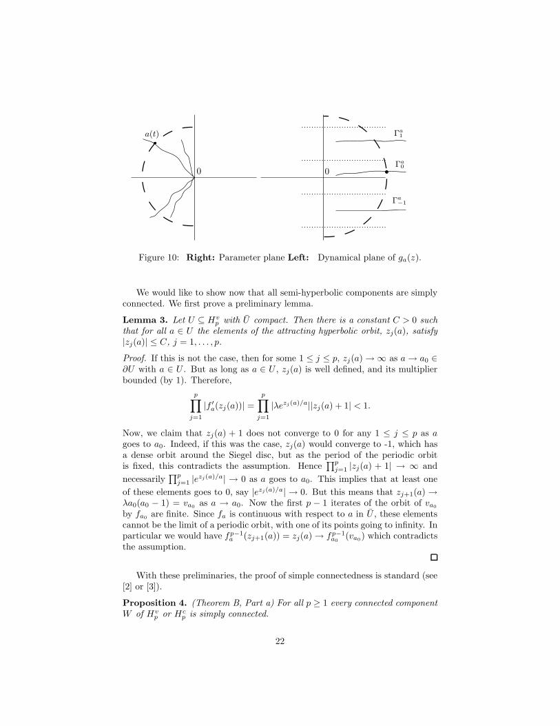
Proposition 3. If γ is a closed curve contained in a component W of Hc∪Cc,then ind(γ, 0) = 0.

Proof. We shall show that there exists a continuous curve a(t) such that fna(t)(−1)n→∞−→

∞ for all t. It then follows that a(t) would intersect any curve γ surroundinga = 0. But if γ ⊂ Hc ∪ Cc, this is impossible. For a 6= 0 we conjugate fa byu = z/a and obtain the family ga(u) = λ(eu(au+ 1− a)− 1 + a). Observe thatg0(u) = λ(eu − 1). The idea of the proof is the following. As a approaches 0,the dynamics of ga converge to those of g0. In particular we find continuousinvariant curves Γak(t), k ∈ Zt∈(0,∞) (Devaney hairs or dynamic rays) such

that Re Γak(t)t→∞−→ ∞ and if z ∈ Γak(t) then Re gna (z) → ∞. These invariant

curves move continuously with respect to the parameter a, and they change lessand less as a approaches 0, since ga converges uniformly to g0.

On the other hand, the critical point of ga is now located at ca = −1/a.Hence, when a runs along a half circle around 0, say ηt = teiα, π/2 ≤ α ≤3π/2, ca runs along a half circle with positive real part, of modulus |ca| = 1/t.

If t is small enough, this circle must intersect, say, Γa0 in at least one point.

This means that there exists at least one a(t) ∈ ηt such that gna(t)(ca(t)n→∞−→ ∞).

Using standard arguments (see for example [8]) it is easy to see that we can

choose a(t) in a continuous way so that a(t)t→0−→ 0. Undoing the change of

variables, the conclusion follows.

21

a(t)

0 0Γa

0

Γa

1

Γa

−1

Figure 10: Right: Parameter plane Left: Dynamical plane of ga(z).

We would like to show now that all semi-hyperbolic components are simplyconnected. We first prove a preliminary lemma.

Lemma 3. Let U ⊆ Hvp with U compact. Then there is a constant C > 0 such

that for all a ∈ U the elements of the attracting hyperbolic orbit, zj(a), satisfy|zj(a)| ≤ C, j = 1, . . . , p.

Proof. If this is not the case, then for some 1 ≤ j ≤ p, zj(a) → ∞ as a → a0 ∈∂U with a ∈ U . But as long as a ∈ U , zj(a) is well defined, and its multiplierbounded (by 1). Therefore,

p∏

j=1

|f ′a(zj(a))| =

p∏

j=1

|λezj(a)/a||zj(a) + 1| < 1.

Now, we claim that zj(a) + 1 does not converge to 0 for any 1 ≤ j ≤ p as agoes to a0. Indeed, if this was the case, zj(a) would converge to -1, which hasa dense orbit around the Siegel disc, but as the period of the periodic orbitis fixed, this contradicts the assumption. Hence

∏pj=1 |zj(a) + 1| → ∞ and

necessarily∏pj=1 |e

zj(a)/a| → 0 as a goes to a0. This implies that at least one

of these elements goes to 0, say |ezj(a)/a| → 0. But this means that zj+1(a) →λa0(a0 − 1) = va0 as a → a0. Now the first p − 1 iterates of the orbit of va0

by fa0 are finite. Since fa is continuous with respect to a in U , these elementscannot be the limit of a periodic orbit, with one of its points going to infinity. Inparticular we would have fp−1

a (zj+1(a)) = zj(a) → fp−1a0

(va0) which contradictsthe assumption.

With these preliminaries, the proof of simple connectedness is standard (see[2] or [3]).

Proposition 4. (Theorem B, Part a) For all p ≥ 1 every connected componentW of Hv

p or Hcp is simply connected.

22

Proof. Let γ ⊂ W a simple curve bounding a domain D. We will show thatD ⊂ W . Let gn(a) = fnpa (va) (resp. fnpa (−1)). We claim that gnn∈N is afamily of entire functions for a ∈ D. Indeed, fa(va) has no essential singu-larity at a = 0 (resp. fa(−1) has no essential singularity as 0 /∈ D), neitherdo fna (fa(va)), n ≥ 1 (resp. fna (fa(−1)), n ≥ 1) as the denominator of theexponential term simplifies.

By definition W is an open set, therefore there is a neighbourhood γ ⊂ U ⊂W . By Lemma 3 |zj(a)| < C, j = 1, . . . , p and it follows that gn(a)n∈N isuniformly bounded in U , since it must converge to one point of the attractingcycle as n goes to ∞. So by Montel’s theorem and the Maximum ModulusPrinciple, this family is normal, and it has a sub-sequence convergent in D.If we denote by G(a) the limit function, G(a) is analytic and the mappingH(a) = fpa (G(a))−G(a) is also analytic. By definition of Hp, H(a) is identicallyzero in U , and by analytic continuation it is also identically zero inD. ThereforeG(a) = z(a) is a periodic point of period p.

Now let χ(a) be the multiplier of this periodic point of period p. Thismultiplier is an analytic function which satisfies |χ(a)| < 1 in U , and by theMaximum Modulus Principle the same holds in D. Hence D ⊂ Hv

p (resp.D ⊂ Hc

p).

The following lemma shows that the asymptotic value itself can not be partof an attracting orbit.

Lemma 4. There are neither a nor p such that fp(va) = va and the cycle isattracting.

Proof. It cannot be a super-attracting cycle since such orbit must contain thecritical point and its forward orbit, but the critical orbit is accumulating on theboundary of the Siegel disc and hence its orbit cannot be periodic.

It cannot be attracting either, as the attracting basin must contain a singularvalue different from the attracting periodic point itself, and this could only bethe critical point. But, as before, the critical point cannot be there. Theconclusion then follows.

We can now show that all components in Hvp are unbounded, which is part

of Part b) of Theorem B. The proof is also analogous to the exponential case(see [2] or [3]).

Theorem 4.21. Every connected component W of Hvp is unbounded for p ≥ 1.

Proof. From Lemma 3 above, the attracting periodic orbit z(a) of Proposition4 above is not only analytic in W but as lim sup|χ(a)| ≤ 1 for a ∈ W , z(a)has only algebraic singularities at b ∈ ∂W . These singularities are in fact pointswhere χ(b) = 1 by the implicit function theorem. This entails that the boundaryof W is comprised of arcs of curves such that |χ(a)| = 1.

23

The multiplier in W is never 0 by Lemma 4, thus if W is bounded, it is acompact simply-connected domain bounded by arcs |χ(a)| = 1. Now ∂χ(W ) ⊂χ(∂W ) ⊂ χ||χ| = 1 but by the minimum principle this implies 0 ∈ χ(W )against assumption.

To end this section we show the existence of the largest semi-hyperboliccomponent, the one containing a segment [r,∞) for r large, which is TheoremB, Part c).

Theorem 4.22. The parameter plane of fa(z) has a semi-hyperbolic componentHv

1 of period 1 which is unbounded and contains an infinite segment.

Proof. The idea of the proof is to show that for a = r > 0 large enough thereis a region R in dynamical plane such that fa(R) ⊂ R. By Schwartz’s lemmait follows that R contains an attracting fixed point. By Theorem 3.19 the orbitof va must converge to it. Not to break the flow of exposition, the detailedestimates of this proof can be found in the Appendix.

Remark 6. The proof can be adapted to the case λ = ±i showing that Hv1 con-

tains an infinite segment in iR. Observe that this case is not in the assumptionsof this paper since z = 0 would be a parabolic point.

4.1 Parametrisation of Hv

p: Proof of Theorem B, Part b

In this section we will parametrise connected components W ⊂ Hvp by means

of quasi-conformal surgery. In particular we will prove that the multiplier mapχ : W → D∗ is a universal covering map by constructing a local inverse of χ.The proof is standard.

Theorem 4.23. Let W ⊂ Hvp be a connected component of Hv

p and D∗ be thepunctured disc. Then χ : W → D∗ is the universal covering map.

Proof. For simplicity we will consider W ⊂ Hv1 in the proof. Take a0 ∈ W ,

and observe that fna (va) converges to z(a) as n goes to ∞, where z(a) is anattracting fixed point of multiplier ρ0 < 1. By Konigs theorem there is aholomorphic change of variables

ϕa0 : Ua0 → D

conjugating fa0(z) to mρ0(z) = ρ0z where Ua0 is a neighbourhood of z(a0).Now choose an open, simply connected neighbourhood Ω of ρ0, such that

Ω ⊂ D∗, and for ρ ∈ Ω consider the map

ψρ : Aρ0 // Aρ

reiζ // rαei(ζ+β log r),

24

where Ar denotes the standard straight annulus Ar = z|r < |z| < 1 and

α =log |ρ|

log |ρ0|, β =

arg ρ− arg ρ0

log |ρ0|.

This mapping verifies ψρ(mρ0(z)) = mρ(ψρ(z)) = ρψρ(z). With this equa-tion we can extend ψρ to mρ(Aρ),m

2ρ(Aρ), . . . and then to the whole disc D by

setting ψ(0) = 0. Therefore, the mapping ψρ maps the annuli mkρ(Aρ) homeo-

morphically onto the annuli z||ρk+1| ≤ |z| ≤ ρk.This mapping has bounded dilatation, as its Beltrami coefficient is

µψρ=α+ iβ − 1

α+ iβ + 1e2iζ .

Now define Ψρ = ψρϕa0 , which is a function conjugating fa0 quasi-conformallyto ρz in D.

Let σρ = Ψ∗ρ(σ0) be the pull-back by Ψρ of the standard complex structure

σ0 in D. We extend this complex structure over Ua0 to f−na0

(Ua0) pulling backby fa0 , and prolong it to C by setting the standard complex structure on thosepoints whose orbit never falls in Ua0 . This complex structure has boundeddilatation, as it has the same dilatation as ψρ. Observe that the resultingcomplex structure is the standard complex structure around 0, because no pre-image of Ua0 can intersect the Siegel disc.

Now apply the Measurable Riemann Mapping Theorem (with dependenceupon parameters, in particular with respect to ρ) so we have a quasi-conformalintegrating map hρ (which is conformal where the structure was the standardone) so that h∗ρσ0 = σρ. Then the mapping gρ = h f h−1 is holomorphic asshown in the following diagram:

(C, σρ′ )ψfaψ

−1

//

hρ′

(C, σρ′ )

hρ′

(C, σ0)gρ′

// (C, σ0)

Moreover, the map ρ 7→ hρ(z) is holomorphic for any given z ∈ C since thealmost complex structure σρ depends holomorphically on ρ. We normalise thesolution given by the Measurable Riemann Mapping Theorem requiring that -1,0 and ∞ are mapped to themselves. This guarantees that gρ(z) satisfies thefollowing properties:

• gρ(z) has 0 as a fixed point with rotation number λ, so it has a Siegel discaround it,

• gρ(z) has only one critical point, at -1 which is a simple critical point,

• gρ(z) has an essential singularity at ∞,

• gρ(z) has only one asymptotic value with one finite pre-image.

25

Moreover gρ(z) has finite order by Theorem 2.4. Then Theorem 3.18 impliesthat gρ(z) = fb(z) for some b ∈ C∗. Now let’s summarise what we have done.

Given ρ in Ω ⊂ D∗ we have a b(ρ) ∈ W ⊂ Hv1 such that fb(ρ)(z) has a

periodic point with multiplier ρ. We claim that the dependence of b(ρ) withrespect to ρ is holomorphic. Indeed, recall that va has one finite pre-image,a− 1. Hence hρ(a− 1) = b(ρ) − 1 which implies a holomorphic dependence onρ.

We have then constructed a holomorphic local inverse for the multiplier. Asa consequence, χ : H → D∗ is a covering map and as W is simply connectedby Proposition 4 and unbounded by Theorem 4.21, χ is the universal coveringmap.

4.2 Parametrisation of Hc

p: Proof of Theorem B, Part d

Let W be a connected component of Hcp which is bounded and simply connected

by Theorem 3.19. The proof of the following proposition is analogous to thecase of the quadratic family but we sketch it for completeness.

Proposition 5. The multiplier χ : W → D is a conformal isomorphism.

Proof. Let W ∗ = W\χ−1(0). Using the same surgery construction of the previ-ous section we see that there exists a holomorphic local inverse of χ around anypoint ρ = χ(z(a)) ∈ D∗, a ∈W ∗. It then follows that χ is a branched covering,ramified at most over one point. This shows that χ−1(0) consists of at most onepoint by Hurwitz’s formula.

To show that the degree of χ is exactly one, we may perform a differentsurgery construction to obtain a local inverse around ρ = 0. This surgery usesan auxiliary family of Blaschke products. For details see [4] or [6].

5 Capture components: Proof of Theorem C

A different scenario for the dynamical plane is the situation where one of thesingular orbits is eventually captured by the Siegel disc. The parameters forwhich this occurs are called capture parameters and, as it was the case withsemi-hyperbolic parameters, they are naturally classified into two disjoint setsdepending whether it is the critical or the asymptotic orbit the one which even-tually falls in ∆a. More precisely, for each p ≥ 0 we define

C =⋃

p≥0

Cvp ∪⋃

p≥0

Ccp,

where

Cvp = a ∈ C|fpa (va) ∈ ∆a, p ≥ 0 minimal,

Ccp = a ∈ C|fpa (−1) ∈ ∆a, p ≥ 0 minimal,

26

Observe that the asymptotic value may belong itself to ∆a since it has afinite pre-image, but the critical point cannot. Hence Cc0 is empty.

We now show that being a capture parameter is an open condition. Theargument is standard, but we first need to estimate the minimum size of theSiegel disc in terms of the parameter a. We do so in the following lemma.

Lemma 5. For all a0 6= 0 exists a neighbourhood V of a0 such that fa(z) isunivalent in D(0, R).

Proof. The existence of a Siegel disc around z = 0 implies that there is a radiusR′ such that fa0(z) is univalent in D(0, R′). By continuity of the family fa(z)with respect to the parameter a, there are R > 0, ε > 0 such that fa(z) isunivalent in D(0, R) for all a in the set a| |a− a0| < ε.

Corollary 2. For all a0 6= 0 exists a neighbourhood a0 ∈ V such that ∆a

contains a disc of radiusC

4R

where C is a constant that only depends on θ and R only depends on a0.

Proof. For any value of a the maps fa(z) and fa(z) = 1Rλa(e

Rz/a(Rz+1− a)−

1 + a) are affine conjugate through h(z) = R · z. For |a − a0| < ε, fa(z) isunivalent on D, thus we can apply Theorem 2.10 to deduce that the conformalcapacity κa of the Siegel disc ∆a is bounded from below by a constant C = C(θ).Undoing the change of variables we obtain

Rκ = κa ≥ C(θ)

and therefore, by Koebe’s 1/4 Theorem, ∆a contains a disc of radius C(θ)4R .

Theorem 5.24 ((Theorem C, Part a)). Let a ∈ Cvp (resp. a ∈ Ccp) for somep ≥ 0 (resp. p ≥ 1) which is minimal. Then there exists δ > 0 such thatD(a, δ) ⊂ Cvp (resp. Ccp)

Proof. Let b = fpa (va) ∈ ∆a (resp. b = fpa (−1) ∈ ∆a). Assume b 6= 0, (the caseb = 0 is easier and will be done afterwards). Define the annulus A as the regioncomprised between O(b) and ∂∆a as shown in Figure 11.

Define ψ as the restriction of the linearising coordinates conjugating fa(z)to the rotation Rθ in ∆a, taking A to the straight annulus A(1, ε), where εis determined by the modulus of A. Also define a quasi-conformal mappingφ : A(1, ε) → A(1, ε2) conjugating the rotation Rθ to itself. Let φ be thecomposition φ ψ.

Let µ be the fa invariant Beltrami form defined as the pull-back µ = φ∗µ0

in A and spread this structure to ∪nf−na (A) by the dynamics of fa(z). Finally

define µ = µ0 in C\ ∪n f−n(A). Observe that µ = µ0 in a neighbourhood of 0.Also φ has bounded dilatation, say k < 1, which is also the dilatation of µ.

27

∂∆a

O(b)

A

Figure 11: The annulus A.

Now let µt = t · µ be a family of Beltrami forms with t ∈ D(0, 1/k). Thesenew Beltrami forms are integrable, since ‖µt‖∞ = t‖µ‖ < 1

kk = 1. Thus by theMeasurable Riemann Mapping Theorem we get an integrating map φt fixing0,-1 and ∞, such that φ∗tµ0 = µt. Let f t = φt fa φ

−1t ,

(C, µt)

φt

fa// (C, µt)

φt

(C, µ0)ft

//___ (C, µ0)

Since µt is fa-invariant, it follows that f t(z) preserves the standard complexstructure and hence it is holomorphic by Weyl’s lemma.

Notice also that by Theorem 2.4 in Section 2 f t(z) has finite order. Further-more by the properties of the integrating map and topological considerations, ithas an essential singularity at ∞, a fixed point 0 with multiplier λ and a simplecritical point in -1. Finally, it has one asymptotic value φt(a) with one finitepre-image, φt(a − 1). Hence by Theorem 3.18 f t(z) = fa(t)(z) for some a(t).Now we want to prove that a(t) is analytic. First observe that for any fixedz ∈ C, the almost complex structure µt is analytic with respect to t. Hence,by the MRMT, it follows that t 7→ φt(z) is analytic with respect to t. Now,a − 1 is the finite pre-image of va, so φt(a − 1) = a(t) − 1, and this impliesa(t) = 1 + φt(a− 1), which implies that a(t) is also analytic.

It follows that a(t) is either open or constant. But fa(0) = fa and f1 aredifferent mappings since the annuli φ0(A) = A and φ1(A) have different moduli.Then a(t) is open and therefore a(t), t ∈ D(0, 1/k) is an open neighbourhoodof a which belongs to Cvp (resp. Ccp).

If fpa0(va0) = 0 (resp. fpa0

(−1) = 0), by Lemma 5 and Corollary 2 thereexists an ε > 0 such that for all a close to a0, ∆a0 ⊃ D(0, ε). Hence a smallperturbation of fa0 will still capture the orbit of va0 (resp. -1) as we wanted.

28

The theorem above shows that capture parameters form an open set. Wecall the connected components of this set, capture components, which may beasymptotic or critical depending on whether it is the asymptotic or the criticalorbit which falls into ∆a.

As in the case of semi-hyperbolic components, capture components are sim-ply connected. Before showing that, we also need to prove that no criticalcapture component may surround a = 0. We just state this fact, since the proofis a reproduction of the proof of Proposition 3 above.

Proposition 6. Let γ be a closed curve in W ⊂ Cv. Then ind(γ, 0) = 0.

Proposition 7. (Theorem C, Part b) All connected components W of Cv orCc are simply connected.

Proof. Let W be a connected component of Cv or Cc and γ ⊂W a simple closedcurve. Let D be the bounded component of C\γ. Let U be a neighbourhoodof γ such that U ⊂ W . Then, for all a ∈ U , fna (va) (resp. fna (−1)) belongs to∆a for n ≥ n0, and even more it remains on an invariant curve. It follows thatGvn(a) = fna (va) (resp. Gcn(a) = fna (−1)) is bounded in U for all n ≥ n0.

Since Gvn(a) is holomorphic in all of C (resp. in C∗), we have that Gvn(a)(resp. Gcn(a)) is holomorphic and bounded on D, and hence it is a normalfamily in D. By analytic continuation the partial limit functions must coincide,so there are no bifurcation parameters in D. Hence D ⊂W .

As it was the case with semi-hyperbolic components, it follows from Theorem3.19 that all critical capture components must be bounded, since for |a| large,the critical orbit must accumulate on ∂∆a. This proves Part c) if Theorem C.Among all asymptotic capture components, there is one that stands out in allcomputer drawings, precisely the main component in Cv0 . That is, the set ofparameters for which va itself belongs to the Siegel disc.

We first observe that this component must also be bounded. Indeed, ifva ∈ ∆a then its finite pre-image a−1 must also be contained in the Siegel disc.But for |a| large enough, the disc is contained in D(0, R), with R independentof a (see Theorem 3.19). Clearly Cv0 has a unique component, since va = 0 onlyfor a = 0 or a = 1. This proves Part d) of Theorem C.

The “centre” of Cv0 is a = 1, or the map fa(z) = λzez, for which theasymptotic value v1 = 0 is the centre of the Siegel disc. This map is quite well-known, as it is, in many aspects, the transcendental analogue of the quadraticfamily. It is known, for example that if θ is of constant type then ∂∆a is a quasi-circle and contains the critical point. This type of properties can be extendedto the whole component Cv0 as shown by the following proposition.

Proposition 8. (Proposition E, Part a) If θ is of constant type then for everya ∈ Cv0 the boundary of the Siegel disc is a quasi-circle that contains the criticalpoint.

29

Proof. For a = 1, f1(z) = λzez and we know that ∂∆a is a quasi-circle thatcontains the critical point (see [10]). Define cn = fn1 (−1), denote by Oa(−1)the orbit of -1 by fa(z) and

H : cnn≥0 × Cv0 // C

(cn , a) // fna (−1)

Then this mapping is a holomorphic motion, as it verifies

• H(cn, 1) = cn,

• it is injective for every a, as if va ∈ Cv0 , then Oa(−1) must accumulate on∂∆a. Hence fna (−1) 6= fma (−1) for all n 6= m.

• It is holomorphic with respect to a for all cn, an obvious assertion as longas 0 /∈ Cv0 which is always true.

Now by the second λ-lemma (Lemma 2 in Section 2), it extends quasi-conformallyto the closure of cnn∈N, which contains ∂∆a. It follows that for all a ∈ Cv0 ,the boundary of ∆a satisfies ∂∆a = Ha(∂∆a) with Ha quasi-conformal, andhence ∂∆a is a quasi-circle. Since −1 ∈ ∂∆1, we have that −1 ∈ ∂∆a.

We shall see in the next section that this same argument can be generalisedto other regions of parameter space.

6 Julia stability

The maps in our family are of finite type, hence fa0(z) is J -stable if bothsequences fna (−1)n∈Z and fna (va)n∈Z are normal for a in a neighbourhoodof a0 (see [16] or [7]).

We define the critical and asymptotic stable components as

Sc = a ∈ C|Gcn(a) = fna (−1) is normal in a neighbourhood of a,

Sv = a ∈ C|Gvn(a) = fna (va) is normal in a neighbourhood of a,

respectively. Accordingly we define critical and asymptotic unstable componentsUc, Uv as their complements, respectively. These stable components are bydefinition open, its complements closed. With this notation the set of J -stableparameters is then S = Sc ∩ Sv.

Capture parameters and semi-hyperbolic parameters clearly belong to Sc orSv. Next, we show that, because of the persistent Siegel disc, they actuallybelong to both sets.

Proposition 9. Hc,v, Cc,v ⊂ S

30

Proof. Suppose, say, that a0 ∈ Hv. The orbit of va0 tends to an attractingcycle, and hence a0 ∈ Sv. In fact, since Hv is open, we have that a ∈ Sv forall a in a neighbourhood U of a0. For all these values of a, the critical orbitis forced to accumulate on ∂∆a, hence fna (−1)n∈N avoids, for example, allpoints in ∆a. It follows that fna (−1)n∈N is also normal on U and thereforea0 ∈ Sc. The three remaining cases are analogous.

Any other component of S not in H or C will be called a queer component,in analogy to the terminology used for the Mandelbrot set. We denote by Q theset of queer components, so that S = H ∪ C ∪Q.

At this point we want to return to the proof of Proposition 8, where weshowed that, for parameters inside Cv0 , the boundary of the Siegel disc wasmoving holomorphically with the parameter. In fact, this is a general fact forparameters in any non-queer component of the J -stable set.

Proposition 10. Let W be a non-queer component of S = Sc∩Sv, and a0 ∈ W .Then there exists a function H : W × ∂∆a0 → ∂∆a which is a holomorphicmotion of ∂∆a0 .

Proof. SinceW is not queer, we have thatW ⊂ H∪C. Let sa denote the singularvalue whose orbits accumulates on ∂∆a for a ∈ W , so that sa ∈ −1, va. Letsna = fna (sa), and denote the orbit of sa by Oa(sa). Then the function

H : Oa0(sa0) ×W // C

(sna0, a) // sna

is a holomorphic motion, since Oa(sa) must be infinite for all n, and fna (sa) isholomorphic on a, because 0 /∈ W . By the second λ-lemma, H extends to theclosure of Oa0(sa0) which contains ∂∆0.

Combined with the fact that fa(z) is a polynomial-like map of degree 2 for|a| > R (see Theorem 3.19) we have the following immediate corollary.

Corollary 3. (Proposition E, Part b) Let W ⊂ Hv ∪ Cv be a component in-tersecting |z| > R where R is given by Theorem 3.19 (in particular this issatisfied by any component of Hv). Then,

a) if θ is of constant type, for all a ∈ W , the boundary ∂∆a is a quasi-circlecontaining the critical point.

b) Depending on θ ∈ R\Q, other possibilities may occur: ∂∆a might be a quasi-circle not containing the critical point, or a C n, n ∈ N Jordan curve not beinga quasi-circle containing the critical point, or a C n, n ∈ N Jordan curvenot containing the critical point and not being a quasi-circle. In general,any possibility realised by a quadratic polynomial for some rotation numberand which persists under quasi-conformal conjugacy, is realised for somefa = e2πθia(ez/a(z + 1 − a) + a− 1).

31

Remark 7. In general, for any W ⊂ Hv ∪ Cv we only need one parametera0 ∈W for which one of such properties is satisfied, to have it for all a ∈W .

Proof of Theorem 4.22 and numerical boundsWe may suppose λ 6= ±i since θ 6= ±1/2. Let λ = λ1 + iλ2, σ = Sign (λ1)

and ρ = Sign (λ2). We define:

yC2

va

C1

s

C3−y

f(R)

R

Figure 12: Sketch of the construction in Thm. 4.22 for the case λ1, λ2 > 0.

C1 : = σs+ ti||t| ≤ y

C2 : = σt+ iρy|t ≥ s

C3 : = σt− iρy|t ≥ s

with y > 0, s > 0, see Figure 12 for a sketch of this curves. Let R be the regionbounded by C1, C2, C3. Recall that va = λ(a2 − a) is the asymptotic value.Note that we will consider a real, furthermore following Figure 12, we will seta := −σb with b > 0, as hinted by numerical experiments. Defined this way, thecurves that are closer to va are C1 and C2. We choose y and s in such a waythat d(va, C1) = d(va, C2), as in Figure 12. More precisely,

d(va, C1,2) = |λ1|(b2 + σb

)− s = |λ2|(b

2 + σb) − y

and hencey = (|λ1| + |λ2|)

(b2 + σb

)− s.

To ease notation, define L = (|λ1| + |λ2|). We would like some conditions over sassuring that if b > b∗, d(va, f(∂R)) ≤ d(va, ∂R), as this would imply f(R) ⊂ Rand thus the existence of an attracting fixed point. We write fa(z) = va+ ga(z)where ga(z) = a · λez/a · (z + 1 − a). Then

d(va, f(∂R)) = d(0, ga(∂R)) = |ga(∂R)|.

32

Therefore we need to find values such that the following three inequalities hold

|ga(C1)| < |λ1|(b2 + σb

)− s, (6)

|ga(C2)| < |λ1|(b2 + σb

)− s, (7)

|ga(C3)| < |λ1|(b2 + σb

)− s. (8)

For (6) to hold the following inequality needs to be satisfied

b · e−s/b√

((σs+ σb + 1) + t2)?≤ |λ1|

(b2 + σb

)− s.

Observe that

b · e−s/b√

(σs+ σb + 1)2 + t2 ≤ b · e−s/b (|σ(s+ b) + 1| + y) =

= b · e−s/b (s+ b+ σ + y) =

= b · e−s/b(b+ σ + L(b2 + σb)

),

so we define the following function

h(s) = b · e−s/b(b + σ + L(b2 + σb)

)− |λ1|

(b2 + σb

)+ s,

and we will find an argument which makes it negative. We need to find s suchthat h(s) < 0 and 0 < s < |λ1|(b2 + σb)|. It is easy to check that h(s) has alocal minimum at s∗ := b log

(b+ σ + L(b2 + σb)

)and furthermore

h(s∗) = b+ b log(b+ σ + L(b2 + σb)

)− |λ1|

(b2 + σb

),

which is negative for some b∗ big enough (in Appendix 6 we will give someestimates on how big this b∗ must be as a function of λ). This s∗ is again in ourtarget interval, for a big enough b (note that if h(s∗) < 0 then s∗ < |λ1|(b

2+σb)|).From now on, let s = s∗, and check if (7) holds, where we will put s = s∗ at

the end of the calculations.

b · e−σt/σb√

((σt+ σb + 1) + y2)?≤ |λ1|

(b2 + σb

)− s.

As we have done before, expand

b · e−σt/σb√

((σt+ σb + 1) + y2) ≤ b · e−t/b · (|σt+ σb+ 1| + y) =

= b · e−t/b · (t+ b+ σ + y) =

= b · e−t/b ·(t+ b+ σ + L

(b2 + σb

)− s∗

).

It is easy to check that b · e−t/b · (b + σ + y) is a decreasing function in t,and b · e−t/bt has a local maximum at t = b and is a decreasing function fort > b. Then, we can bound both terms by setting t = s∗, as s∗ ≥ b wheneverb+σ+L(b2+σb) is bigger than e, but this inequality holds if all other conditionsare fulfilled. Now we must only check if

|λ1|(b2 + σb

)− s∗

?≥ b · e−s

∗/b ·(s∗ + b+ σ| + L

(b2 + σb

)− s∗

)=

= b ·b + σ + L

(b2 + σb

)

b+ σ + L (b2 + σb)= b,

33

which is the same inequality we have for h(s), thus it is also satisfied. Inequality(8) is equivalent to (6), hence the result follows.

Now we give numerical bounds for how big b must be in Theorem 4.22. Wewill consider only the general case λ1 6= 0, as the other is equivalent.

Consider the inequality

b log(b+ σ + L(b2 + σb

)) ≤ −b+ |λ1|

(b2 + σb

)

If this inequality holds and b+σ+L(b2+σb) > 0, we have the required estimatesto guarantee that all required inequalities in Theorem 4.22 hold. The secondinequality is clearly trivial, as it holds when b > 1. Now, we must find a suitableb for the first.

Simplifying a b factor and taking exponentials in both sides, we must checkwhich b verify

b+ σ + L(b2 + σb) ≤ e−1+|λ1|σe|λ1|b. (9)

We can get a lower bound of ex:

e|λ1|b ≥ 1 + |λ1|b +|λ1|2b2

2+

|λ1|3b3

6.

And this way if

b+ σ + L(b2 + σb) ≤ e−1+|λ1|σ(

1 + |λ1|b +|λ1|2b2

2+

|λ1|3b3

6

),

then is also true (9). Now we must check when a degree 3 polynomial withnegative dominant term has negative values. This will be true as long asb > 0 is greater than the root with bigger modulus. It is well-known (see

[13]) that a monic polynomial zn +∑n−1i aiz

i has its roots in a disc of radius

max(1,∑n−1

i |ai|), so every b > 1 and bigger than

6

eσ|λ1|−1|λ1|3·

(|L− eσ|λ1|−1 |λ1|2

2| + |1 − eσ|λ1|−1|λ1|b + Lσb| + |b+ σ − 1|

)

satisfies our claims.Finer estimates for b depending on λ can be obtained with a more careful

splitting of λ space, for instance

λ|λ ∈ S1 = λ ∈ [7π/4, π/4] ∪ λ ∈ [π/4, 3π/4] ∪ λ ∈ [3π/4, 5π/4]

∪ λ ∈ [5π/4, 7π/4] = B1 ∪B2 ∪B3 ∪B4.

The proof can be adapted with very minor changes to this partition, althoughthe exposition and calculations are more cumbersome.

34

Acknowledgements

The authors wish to thank Xavier Buff and Lasse Rempe for helpful conver-sations. Both authors were partially supported by Spanish grant MICINNMTM2006-05849/Consolider and European funds MCRTN-CT-2006-035651. Thesecond author was also partially supported by Spanish grant MICINN MTM2008-01486 and by Catalan grant CIRIT 2005/SGR01028.

References

[1] Lars V. Ahlfors. Lectures on quasiconformal mappings, volume 38 of Uni-versity Lecture Series. American Mathematical Society, Providence, RI,second edition, 2006. With supplemental chapters by C. J. Earle, I. Kra,M. Shishikura and J. H. Hubbard.

[2] I. N. Baker and P. J. Rippon. Iteration of exponential functions. AnnalesAcademiae Scientiarum Fennicae Series A I Mathematica, 9:49–77, 1984.

[3] Clara Bodelon, Robert L. Devaney, Michael Hayes, Gareth Roberts, Lisa R.Goldberg, and John H. Hubbard. Hairs for the complex exponential family.International Journal of Bifurcation and Chaos in Applied Sciences andEngineering, 9(8):1517–1534, 1999.

[4] Bodil Branner and Nuria Fagella. Quasiconformal surgery in holomorphicdynamics. Work in progress.

[5] John B. Conway. Functions of one complex variable, volume 11 of GraduateTexts in Mathematics. Springer-Verlag, New York, second edition, 1978.

[6] Adrien Douady. Disques de Siegel et anneaux de Herman. Asterisque,(152-153):4, 151–172 (1988), 1987. Seminaire Bourbaki, Vol. 1986/87.

[7] A. E. Eremenko and M. Yu. Lyubich. Dynamical properties of some classesof entire functions. Annales de l’Institut Fourier. Universite de Grenoble,42(4):989–1020, 1992.

[8] Nuria Fagella. Limiting dynamics for the complex standard family. Inter-national Journal of Bifurcations and Chaos in Applied Sciences and Engi-neering, 5(3):673–699, 1995.

[9] Nuria Fagella, Tere M. Seara, and Jordi Villanueva. Asymptotic size of Her-man rings of the complex standard family by quantitative quasiconformalsurgery. Ergodic Theory and Dynamical Systems, 24(3):735–766, 2004.

[10] Lukas Geyer. Siegel discs, Herman rings and the Arnold family. Transac-tions of the American Mathematical Society, 353(9):3661–3683 (electronic),2001.

35

[11] Lisa R. Goldberg and Linda Keen. A finiteness theorem for a dynamicalclass of entire functions. Ergodic Theory and Dynamical Systems, 6(2):183–192, 1986.

[12] Michael-R. Herman. Are there critical points on the boundaries of singulardomains? Communications in Mathematical Physics, 99(4):593–612, 1985.

[13] Holly P. Hirst and Wade T. Macey. Bounding the roots of polynomials.The College Mathematics Journal, 28(4):292–295, Sept 1997.

[14] R. Mane, P. Sad, and D. Sullivan. On the dynamics of rational maps.Annales Scientifiques de l’Ecole Normale Superieure (4), 16(2):193–217,1983.

[15] Ricardo Mane. On a theorem of Fatou. Boletim de Sociedade Brasileira deMatematica (N.S.), 24(1):1–11, 1993.

[16] Curtis T. McMullen. Complex dynamics and renormalization, volume 135of Annals of Mathematics Studies. Princeton University Press, Princeton,NJ, 1994.

[17] John Milnor. Dynamics in one complex variable, volume 160 of Annalsof Mathematics Studies. Princeton University Press, Princeton, NJ, thirdedition, 2006.

[18] Ricardo Perez-Marco. Fixed points and circle maps. Acta Mathematica,179(2):243–294, 1997.

[19] Lasse Rempe. On a question of Herman, Baker and Rippon concerningSiegel disks. Bulletin of the London Mathematical Society, 36(4):516–518,2004.

[20] Lasse Rempe. Siegel disks and periodic rays of entire functions. Journalfur die reine und angewandte Mathematik, 624:81–102, 2008.

[21] James T. Rogers, Jr. Singularities in the boundaries of local Siegel disks.Ergodic Theory and Dynamical Systems, 12(4):803–821, 1992.

[22] James T. Rogers, Jr. Recent results on the boundaries of Siegel disks. InProgress in holomorphic dynamics, volume 387 of Pitman Research Notesin Mathematical Series, pages 41–49. Longman, Harlow, 1998.

[23] Gunther Rottenfusser. Dynamical fine structure of entire transcendentalfunctions. Doctoral Thesis, International University Bremen, 2005.

[24] Carl Ludwig Siegel. Iteration of analytic functions. Annals of Mathematics(2), 43:607–612, 1942.

[25] Zbigniew Slodkowski. Holomorphic motions and polynomial hulls. Proceed-ings of the American Mathematical Society, 111(2):347–355, 1991.

36

[26] Jean-Christophe Yoccoz. Petits diviseurs en Dimension 1. Number 231 inAsterisque. Societe Mathematique de France, 1995.

[27] Jean-Christophe Yoccoz. Analytic linearization of circle diffeomorphisms.In Dynamical systems and small divisors (Cetraro, 1998), volume 1784 ofLecture Notes in Mathematics, pages 125–173. Springer, Berlin, 2002.

[28] Saeed Zakeri. Dynamics of cubic Siegel polynomials. Communications inMathematical Physics, 206(1):185–233, 1999.

37