Allocating the US Federal Budget to the States: the Impact of the President∗

Valentino Larcinese1

Department of Government and STICERD London School of Economics and Political Science

Leonzio Rizzo

Department of Economics University of Ferrara

Cecilia Testa

Department of Economics Royal Holloway College

Political Economy and Public Policy Series The Suntory Centre Suntory and Toyota International Centres for Economics and Related Disciplines London School of Economics and Political Science Houghton Street London WC2A 2AE

PEPP/3 June 2005 Tel: (020) 7955 6674

∗ Acknowledgements: We wish to thank Tim Besley, Robert Franzese, Jim Snyder and Cristiana Vitale for helpful discussions and suggestions and the participants to seminars at STICERD, Royal Holloway College, Ente Einaudi, LSE, Bocconi University, FGV, USP, LAMES 2004 Santiago, PET04 Beijing, the Public Economics week end at the University of Essex and the 2005 meeting of the Midwest Political Science Association for their useful comments. Remaining errors are only ours. 1 Address for correspondence: London School of Economics, Department of Government, Houghton Street, London, WC2A 2AE, United Kingdom, Tel. +44 (0) 20 7955 6692. Fax: +44 (0) 20 7955 6352. E-mail: V.Larcinese@lse.ac.uk.

Abstract

This paper provides new evidence on the determinants of the US federal budget allocation to the states. Departing from the existing literature that gives prominence to Congress, we carry on an empirical investigation on the impact of Presidents during the period 1982-2000. Our findings suggest that the distribution of federal outlays to the States is affected by presidential politics. First, presidential elections matter. States that heavily supported the incumbent President in past presidential elections tend to receive more funds, while marginal and swing states are not rewarded. Second, party affiliation also plays an important role since states whose governor has the same political affiliation of the President receive more federal funds, while states opposing the president's party in Congressional elections are penalized. These results show that presidents are engaged in tactical distribution of federal funds and also provide good evidence in support of partisan theories of budget allocation. Keywords: Federal Budget, Pork-Barrell, President, Congress, Political Parties, Committees, American Elections. JEL: D72, H61, H70 © The authors. All rights reserved. Short sections of text, not to exceed two paragraphs, may be quoted without explicit permission provided that full credit, including © notice, is given to the source

“For republican governors, it means we have an ear in the White House, we have a

number we can call, we have access that we wouldn’t have otherwise had, and that’s of

course helpful” ( Gov. Mitt Romney, Washington Post, Monday, November 22, 2004)1

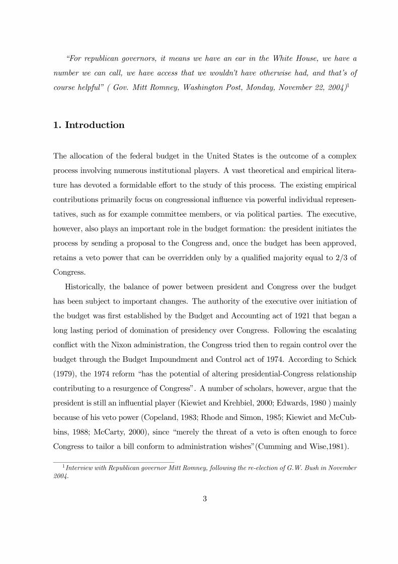
1. Introduction

The allocation of the federal budget in the United States is the outcome of a complex

process involving numerous institutional players. A vast theoretical and empirical litera-

ture has devoted a formidable effort to the study of this process. The existing empirical

contributions primarily focus on congressional influence via powerful individual represen-

tatives, such as for example committee members, or via political parties. The executive,

however, also plays an important role in the budget formation: the president initiates the

process by sending a proposal to the Congress and, once the budget has been approved,

retains a veto power that can be overridden only by a qualified majority equal to 2/3 of

Congress.

Historically, the balance of power between president and Congress over the budget

has been subject to important changes. The authority of the executive over initiation of

the budget was first established by the Budget and Accounting act of 1921 that began a

long lasting period of domination of presidency over Congress. Following the escalating

conflict with the Nixon administration, the Congress tried then to regain control over the

budget through the Budget Impoundment and Control act of 1974. According to Schick

(1979), the 1974 reform “has the potential of altering presidential-Congress relationship

contributing to a resurgence of Congress”. A number of scholars, however, argue that the

president is still an influential player (Kiewiet and Krehbiel, 2000; Edwards, 1980 ) mainly

because of his veto power (Copeland, 1983; Rhode and Simon, 1985; Kiewiet and McCub-

bins, 1988; McCarty, 2000), since “merely the threat of a veto is often enough to force

Congress to tailor a bill conform to administration wishes”(Cumming and Wise,1981).

1Interview with Republican governor Mitt Romney, following the re-election of G.W. Bush in November

2004.

3

In this paper we ask whether the president has a systematic impact on the allocation

of the federal budget to the states. Evidence of presidential influence on the territorial

distribution of federal funds has been provided by several studies on the New Deal pro-

gram. In particular, Wright (1974) and Wallis (1987), have found that states with high

volatility of presidential vote received more federal support, which is consistent with the

idea that the president might try to target swing voters2. On the other hand, Anderson

and Tollison (1991) and Couch and Shughart (1998) find a positive correlation between

Roosvelt share of votes in 1932 and spending at state level3 that is compatible with the

hypothesis of rewarding loyal rather than swing voters. Finally, Fishback et al.. (2003)

and Fleck (2001) find evidence in support of both hypotheses4.

While the New Deal has received great attention, there is a lack of empirical studies

on presidential influence after the 1974 reform. Is the presidential impact still relevant

or does Congress now dominate federal budget allocation? In this paper we attempt to

answer this question by providing new empirical evidence on contemporary federal budget

allocation to the states.

From a theoretical point of view, the executive may have several reasons to sway

the federal budget allocation away from a purely social welfare maximizing objective

(McCarty, 2000). Namely, the president may use budget allocation to enhance his re-

election chances either by targeting swing states or by rewarding his supporters. Lindbeck

and Weibull (1987 and 1993) provide theoretical models explaining why political actors

should redistribute funds to marginal and swing states in order to maximize their chances

of winning elections. Cox and McCubbins (1986) argue instead that, because of the

ideological relationship between voters and candidates, more funds should be allocated

where policy-makers have larger support. In particular, the targeting of loyal voters can

be seen as a safer investment as compared to aiming for swing voters. Hence, risk adverse

political actors that want to maximize the chances of winning elections, should allocate

2Stromberg (2004) shows, however, that these findings are not robust to the inclusion of state fixed

effects.3Anderson and Tollison (1991) also find evidence of committee influence on New Deal Spending.4For an overview of the literature on New Deal spending see Couch and Shughart (1998) and Fishback

et al. (2003).

4

more funds to loyal states. Dixit and Londregan (1996) provide an alternative model

where politician face incentives to target both swing and loyal voters. On the one hand,

moderate voters, who are indifferent between two parties, can more easily be bought; on

the other, core supporters can be targeted in a more efficient way because parties know

their preferences better.

Besides targeting specific groups of voters, the president could also try to further his

legislative agenda by directing spending to specific legislators. Moreover, “as a leader of

his party, he may feel the pressure to favor legislative districts controlled by members

of his party” (McCarty, 2000). Assuming that party reputation is a public good for

individual party members, Cox and McCubbins (1993) provide a theoretical explanation

for cooperation among representatives belonging to the same party5. Along the same

line, Dasgupta et al. (2004), argue that when the electoral returns from spending are

shared between state and central government, then transferring funds to a governor of

the opponent party generates a “leakage” effect whereby the central government looses

part of the electoral benefit from spending. Finally, if state governments have some

discretion in the way funds are spent, then the federal administration could prefer to

allocate more funds to governors with the same policy preferences. All this seems to

suggest that the president has incentives to sway the allocation of federal funds in the

direction of “friendly” administrators.

This study will test these alternative theories of presidential influence. In particular,

we will first estimate the effect of the presidential electoral race on the budget allocation

to find out whether the president rewards his supporters or whether he targets states that

are marginal or swing in presidential elections. Second, to uncover whether the president

diverts federal funds toward states controlled by members of his party, we will estimate

the effect of partisan alignment between the president and the state governors and/or

state representatives.

The impact of the president as a party leader and, more generally, the distributive

5The evidence reported by the media on cooperation between party members is abundant. During

presidential campaigns a huge emphasis is placed, for example, on the ability of governors to deliver the

votes of their state.

5

effects of cooperation between representatives belonging to the same party, are impor-

tant theoretical questions that have not been explored yet by the empirical literature on

partizan budgeting, that tends instead to focus on the role of parties inside Congress.

Among the contributions on congressional partizan budgeting, Levitt and Snyder (1995)

find that, when Congress was dominated by democratic majorities, outlays at the district

level were positively correlated with the district share of democratic votes6. Similarly,

Carsey and Rundquist (1999) find that states represented by Democrats on a defense

committee receive more military procurement awards. Bickers and Stein (2000) find that

the Republican control of the 104th Congress altered the composition of federal outlays

in favor of programs that are more compatible with the interests of Republican represen-

tatives7.

One important advantage of our empirical analysis is that it relies on panel data on

federal outlays over a relatively long time span. The panel structure allows us to use state

fixed effects to account for state-level unobserved heterogeneity and identify the effect of

the relevant political and economic variables8. Since the president, unlike most other

individual players, can exercise his influence on any budgetary aggregate, we decided to

focus our attention on total federal outlays. This approach has its own drawbacks but, for

our purposes, also provides substantial advantages. Focussing on very specific aggregates,

as most literature does, makes it possible to shed light on specific forms of influence

and to be very precise on them. This is particularly true for studies on committees,

where distortions are more often found on specific spending programs. It is, however,

quite possible that the distortions introduced by different actors with limited influence

may offset each other leaving a state without a real advantage in the overall allocation

of federal funds. Since the presidential influence is not limited to particular aggregates,

6Evidence of a bias in favour of democratic districts is also reported by Owens and Wade (1984),

Alvarez and Saving (1997) and Kiewiet and McCubbins (1985). Some recent literature has investigated

the role of parties on budget allocation also in other countries. Dasgupta et al. (2001) find that Indian

states ruled by the same party that controls the central goverment receive more grants, while Dahlberg

and Johansson (2000) find that the Swedish regions that are “swing” in the national elections receive a

higher share of a specific transfer program.7They find, for example, a remarkable increase in the pro-business contingent liabilities.8When data on specific years are used instead, it is hard to say if the results obtained are merely due

to particular features of the data considered or to proper and long lasting political influence.

6

then it is more likely that a state can be favoured in the overall budget allocation for

reasons related to presidential politics. Therefore, total federal spending is the place

where the presidential influence is more likely to be detected. Focussing on whether a

state receives, on aggregate, more federal funds we are of course capturing only a particular

channel through which political actors may divert funds toward their constituencies. The

composition of the budget is another instrument that can be used to favour interests

located in a given constituency, as it is shown by Bickers and Stein (2000).

While we are primarily interested in the role of the president, we also incorporate

into the analysis the other relevant institutional players (Congress and committees) be-

cause excluding some explanatory variables in the regressions may lead to the well known

problem of omitted variable bias9. Therefore, we check the robustness of our results by

simultaneously estimating in the same regressions the impact of several channels of po-

litical influence that, according to previous studies, may crucially affect federal budget

allocation. Following Atlas et al. (1995) and Lee (1998), we control for overrepresenta-

tion of small states in Congress. Furthermore, individual representatives occupying key

positions in the budget process can convey disproportionate amount of money to their

districts (Fenno 1973, Kiewiet and McCubbins, 1988) and according to several scholars,

committees are very influential in determining the budget allocation (Shepsle and Wein-

gast 1987) since they have an advantage both in terms of their agenda setting power

(McKelvey and Ordeshook, 1980) and in terms of information and competence10 (Kre-

hbiel, 1991). Hence, we follow the empirical literature on committee influence11 and

introduce committee membership in our analysis.

To briefly summarize our main results, we find that the president has an important

9When different explanatory variables are correlated, as it seems reasonable to expect in most cases,

omitting relevant players could deliver biased estimates of the impact of those considered.10Weingast and Marshall (1988) argue that committees are the devices that make logrolling work, by

facilitating the trade of influence in the absence of a spot market for the exchanging of support.11The empirical literature on committee influence is vast and, although the results are sometimes

mixed, committee influence is usually found on specific spending categories rather than large spending

aggregates. Among the numerous studies on committees see Plott (1968), Goss (1972), Ferejohn (1974),

Ritt (1976), Strom (1975), Rundquist and Griffit (1976), Ray (1981), Kiel and McKinzie (1983), Rich

(1989), Anderson and Tollison (1991), Owens and Wade (1984), Alvarez and Saving (1997), Carsey and

Rundquist (1999), Levitt and Poterba (1999), Aldrich and Rhode (2000) Bond et al. (2004), Knight

(2004). For an overview on the Committee influence literature see Bond et Al (2004).

7

impact on the allocation of the budget to the states. In particular, states that ideologically

lean towards the president, i.e. states with a high share of presidential votes or with a

governor belonging to the party of the president, tend to be rewarded with more funds.

On the other hand, states with a close presidential electoral race and states that either

changed political affiliation in the most recent election or that are historically volatile

do not receive more money. Hence, overall our analysis suggests that the president is a

relevant player as he can direct more funding toward those states that are run by “friendly”

governors and that have large groups of “core supporters”. Finally, our analysis indicates

that partisanship plays an important role since governors politically aligned with the

president receive more resources and Congress members opposing the president bring less

funds to their states.

The remainder of the paper is organized as follows. The next section describes our

dataset and lays out our empirical approach. Section 2 presents our main results. In

section 3 we provide our conclusions.

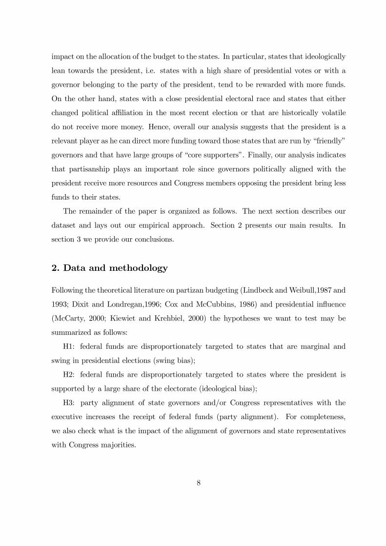
2. Data and methodology

Following the theoretical literature on partizan budgeting (Lindbeck andWeibull,1987 and

1993; Dixit and Londregan,1996; Cox and McCubbins, 1986) and presidential influence

(McCarty, 2000; Kiewiet and Krehbiel, 2000) the hypotheses we want to test may be

summarized as follows:

H1: federal funds are disproportionately targeted to states that are marginal and

swing in presidential elections (swing bias);

H2: federal funds are disproportionately targeted to states where the president is

supported by a large share of the electorate (ideological bias);

H3: party alignment of state governors and/or Congress representatives with the

executive increases the receipt of federal funds (party alignment). For completeness,

we also check what is the impact of the alignment of governors and state representatives

with Congress majorities.

8

We use data on federal outlays for the 48 US continental states from 1982 to 200012.

In Table 1 we report average per capita federal outlays during the period 1982-2000

(expressed in real $ for the year 2000). It is immediately clear that the differences in

spending can be substantial. An average resident of Virginia, for example, has received

every year almost $ 2,700 more than an average resident of Wisconsin. While this gap

can be entirely due to the needs and characteristics of the respective populations, it is

legitimate to ask how much of this difference can be due to purely political factors. For

this purpose we estimate the following equation:

FEDEXPst = αs + βt + θ1Pisw + θZst + st, (1)

s = 1, ...48; t = 1982, ...2000;

where FEDEXPst is the real per-capita federal expenditure (outlays) in state s at time

t. As in all the subsequent regressions, we include state fixed effects and year dummies.

Zst is a vector that includes real income per capita, state population, unemployment rate,

percentage of citizens aged 65 or above and percentage of citizens between 5 and 17 years

old. We keep these explanatory variables in all the regressions as standard economic

and demographic controls. Finally, Pisw represents the set of institutional and political

variables under consideration13.

It is important to point out that in the US budget process there is a lag between

the appropriation of federal funds and the moment when these are actually spent. This

is relevant when estimating the effect of particular institutional and political variables,

since current federal outlays have normally been appropriated in previous budgetary years.

Delays should therefore be taken into account. Hence, we introduce lagged values for Pist,

since past policy makers are responsible for current outlays. To give the right weight

to lagged independent variables explaining current outlays, we use weighted averages of

12As customary, Alaska, District of Columbia and Hawaii have been excluded. Usually those states tend

to be excluded to facilitate comparison with previous research. Another reason, and probably a better

one, however, is that they attract a disproportionate amount of federal spending for either aministrative

reasons (DC) or strategic reasons (Alaska and Hawaii receive a substantial share of defense spending).

This could render the political motivations behind an observed distribution less recognizable.13Summary statistics are reported in the Statistical Appendix.

9

lagged Pis, where the weights are determined by the spend-out rates utilized in official

forecasts. Hence, since we know that approximately 60% of aggregate federal expenditure

is spent within one year, and assuming that the rest is spent two years later, we regress

outlays at time t on the weighted average of two lagged variables, i.e. Pisw = 0.6∗Pi

st−1+

0.4 ∗Pist−2.

Hypotheses 1 and 2. We begin our analysis by considering the role of electoral

competition in the presidential electoral race. Hence, we compare the relative impact of

the closeness of the presidential elections in each state with that of the share of votes

obtained by the president in the last election14. A negative sign of the closeness variable

should be regarded as support for the idea that the president tends to direct resources to

marginal states in order to increase his chances of re-election. A positive sign of the share

of presidential votes should instead be seen as evidence that incumbents tend to reward

states that show their support in elections. We also take into account the fact that not all

states have the same weight in presidential elections by including the number of electoral

votes per capita by state.

The closeness of the past election is, however, not necessarily the best measure to

identify swing states. We, therefore, generate an indicator of long term swing which is

based on the number of times a state swung its support from a party to another in last

four presidential elections15.

Hypothesis 3. As previously discussed, the partisanship of different representatives

can have an important effect on budget allocation since cooperation between different

political actors belonging to the same party is likely to occur. In particular, the president

acting as a party leader may divert funds toward state governors and state representatives

14Hypothesis 1 and 2 are different because, although correlated, the closeness and the presidential share

of votes measure two separate electoral phenomena. First, they can be different when there are more

than two candidates. More importantly, however, they are different because while an electoral race can

be equally "close" in states where the president has won or lost to the opponent, the share of presidential

votes will necessarily be different when the president wins.15We have also used two other measures of electoral volatility. One is a moving average of the frequency

of swings from one party to the other that starts from the 1964 election. The other is an indicator of

short term volatility represented by a dummy equal to one for the states that switched their support in

the last election. Our results do not change when we use such alternative measures. Further details can

be found in the online statistical appendix.

10

belonging to his own party. Hence, we consider a series of dummy variables to capture

various levels of partizan alignment between central powers and state governments. We

first create three dummy variables to reflect the political alignment of state governors

with, respectively, the president and the majorities in the House and in the Senate. In a

further specification we also consider the possibility that funds allocation to a given state

is facilitated by party alignment between the governor and the majority of state delegates

to the House or the governor and both senators. We then consider the potential effect of

having the president and a majority of state delegates in the House, or the president and

both senators from a given state, belonging to the same party. Finally, we consider the

potential advantage of having a majority of state delegates to the House belonging to the

House majority party or having both senators belonging to the Senate majority.

We are aware that testing our hypotheses separately has a major limitation because,

by considering one element at time, we can miss relevant correlations and incorrectly

estimate some effects. For this reason we run a regression including all the Pisw vectors

in one equation of the form:

FEDEXPst = αs + βt +Xi

θi1Pist + θ2Zst + st, (3)

The results we get from equation (3) provide the big picture that is missed when

focussing on specific channels of influence and provide an important robustness check.

3. Results

3.1. Swing and Ideological Bias

In Table 2 we focus on presidential elections to test the swing voter hypothesis and contrast

it with the potential presence of ideological bias. Column 1 shows that, while the share

of presidential votes in the past election displays a positive and significant coefficient, the

closeness of the same election has no significant effect16. In column 2 we consider the swing

16Concerning the economic variables, states with higher income per-capita receive significantly less, as

do states with larger population. The percentage of aged population also has a positive and significant

11

variable and we find again no evidence in support of the swing voter hypothesis, while the

share of presidential vote has always a positive and significant effect17. Depending on the

specification considered, the difference in spending between a state with maximum share

of presidential vote and a state with the minimum of such share goes from $536 (column

1) to $908 (column 2) per capita per year, which implies that one standard deviation in

the share of presidential vote is worth 97-164 $. These findings are in line with some of the

existing literature. For example, Anderson and Tollison (1991) and Couch and Shughart

(1998) find a positive correlation between spending at the state level and Roosvelt share

of votes in 1932, and Wright (1974) finds no effect of the closeness of the presidential

race18.

To summarize, we find that the ideological bias toward safe states is substantial in

terms of both magnitude and statistical significance. We do not find instead any evidence

of the refined targeting of swing and marginal states that some formal models seem to

suggest. Assuming that electors cast their vote depending on the amount of spending

they receive and also on their ideological affinity to a party, the swing voter bias should

come from the fact that moderate voters (who are indifferent between two parties) can be

more easily convinced to switch their vote in favor of the party that has rewarded them

with spending. However, as Dixit and Londregan (1996) point out, the electoral return

from a dollar of spending is higher when targeted to an electorate whose preferences the

politician understands well. Hence, although the vote of the moderate electors may be

“cheaper” to buy, the informational advantage and ability of parties to target funds more

efficiently to their supporters can explain why allocating more spending to states with

effect. The percentage of children in schooling age has instead a negative and significant effect, while

the unemployment rate is completely uncorrelated with aggregate spending per capita. The signs and

significance of those coefficients remain substantially the same in all the subsequent specifications.17One obvious concern is that the significance of our estimates could be heavily conditioned by mul-

ticollinearity among the independent variables. To verify that the correlations of our predictors do not

significantly inflate the estimation of their standard errors, we calculate the Variance Inflation Factor for

all the regressions we present in this work. Here, as well as all the subsequent regressions, we find that

that multicollinearity has a very limited impact on the results of all the regressions. A description of the

methodology and detailed results are reported in the statistical appendix.18Our results are also consistent with the findings of Stromberg (2004), who shows how, when state

fixed effects are included in the regressions, evidence that swing states received more federal support

under the New Deal vanishes.

12

many loyal voters can deliver a better electoral return than targeting areas with many

swing voters.

3.2. Party Alignment

In this section we explore the effect of partizan alignment between central and state

government. Our analysis provides support for the idea that partisanship matters and

that political actors exchange favors and policies within the party boundaries. Column

1 of Table 3 shows that the coefficient of the alignment between the president and the

governor in a given state has a positive and statistically significant impact. The size of

the coefficient is also relevant, implying a transfer of approximately 135-138 $ per capita

per year. On the other hand, we find that the effect of alignment of governors with the

majority in either chamber of Congress is not significant. This is especially important

because it shows both the relevance of party affiliation at different levels of governance

and the prominent role of the president in the budget process as a party leader.

In column 2, we include other alignment variables. The significance and magnitude of

the alignment between governors and the president appears unaffected by the introduction

of new variables. Other alignment variables appear to have no statistically significant

impact. The only exception is represented by having a majority of state delegates to

the House belonging to the same party of the president. This again suggests that the

widespread emphasis on the role of the House in the allocation of the federal budget can

obscure the important role played by both the president and the party affiliation19.

The role of parties in American politics has been reconsidered in recent research and

new evidence about party cohesion casts some doubts on the common view that American

parties are weak organizations, with limited ideological divide (Rohde, 1991). If parties are

influential, then the president, as a party leader, may favor legislative districts controlled

19To take into account possible multicollinearity we also run separate regressions for different forms

of alignment. The results (available in the online statistical appendix) remain unchanged, with the

exception of the alignment between the majority of state delegates and the House Majority, which has

now a negative impact. This is not surprising if we consider that the House has been mostly opposed

to the president in the period we consider (with the exception of the period 1993-94). To confirm this,

when we directly include alignments with the President (column 2 of Table 3), this result vanishes.

13

by members of his party. By showing that the president is able to target more funds toward

states that are controlled by state governors belonging to his party, we find good evidence

in support of the theoretical literature that gives prominence to political parties and party

leaders in shaping public policies. Consistently with Levitt and Snyder (1995), who find

that democratic districts received more federal spending under the Carter administration

than under the Reagan administration, we also find that state representatives opposing

the president bring less funds to their states as compared to representatives aligned with

the president.

For what concerns the relationship between the president and the state governors,

Carsey and Wright (1998) find that votes in gubernatorial elections crucially depend on

presidential approval rate. On the other hand, governors can play an important role in

presidential elections as suggested by the attention the media devote to the ability of state

governors to “deliver” the vote of their state. The casual evidence on the privileged par-

tizan link between president and governors is abundant20. The endorsement of governors

also plays a fundamental role in the selection of presidential candidates during primaries21

and the governors associations underline their important role in shaping federal policies22.

Uncovering that the partisanship of state governors and president is an important deter-

minant of the distribution of federal funds to the states, our study provides evidence of

an effective link between governors and the president through political parties.

3.3. Robustness

We now check if our results are robust to a different specification, in which various effects

are considered at the same time. In Table 4 we test simultaneously the different, though

20In a recent interview, following the recent US presidential election of 2004, Mitt Romney, Governor

of Massachussets declared that “for republican governors, it means we have an ear in the White House,

we have a number we can call, we have access that we wouldn’t have otherwise had, and that’s of course

helpful” (Gov. , Washington Post, Monday, November 22, 2004)21The Republican Governors’ Association reports that “Presidential candidates hailing from out of state

can trade on a governor’s name cachet and fund-raising network, while governors can gain a powerful

ally in the Oval Office if their horse wins the race” (Larry Sabato on interview the by Kenneth P.

Vogel,Wednesday June 18, 2003, The News Tribune).22Both the Republican and Democratic Governors’ Associations explicitely state on their website their

intent to influence federal policies.

14

not necessarily conflicting, hypotheses.

From columns 1 it is clear that all the results previously obtained on individual vari-

ables (or group of variables) are substantially confirmed by this check. In particular, the

share of votes for the president and the party alignment between the president and the

governors have a positive impact and are statistically significant at the 5% level. The

alignment of the president with the majority of state delegates in the House is positive

and significant at 10% level. As discussed in the previous section, many reasons can in-

duce a president to support friendly governors. To shed further light on this relationship,

in column 2 we introduce a dummy equal to 1 if the state has a gubernatorial election

in a given year and we also interact this dummy with the governor-president alignment

variable. If the president supports the re-election prospects of friendly governors then the

interaction term should be positive. This turns out to be the case: while the size and sig-

nificance of all other variables are only marginally affected, presidents appear to support

friendly governors particularly in their re-election years. This corroborates our findings

about both the presidential pork-barrel and the privileged relationship with governors

from the same party.

In column 3 we add a number of further controls that previous studies have identified

as determinants of the federal budget allocation. We consider the role of committee

membership, focussing on the most influential committees in the budget process. We use

as explanatory variables the number of members by state in the Appropriation, Budget,

Ways and Means, and Rules committees of the House. We also include the electoral

turnout in presidential elections and a dummy variable for having a democratic president.

To take into account overrepresentation we follow Atlas et al. (1995) and introduce the

number of senators per capita. We find that having a democratic president substantially

increases overall spending (more than 1000 $ yearly per capita). Overrepresentation is

positive and significant23. We do not find any evidence that turnout has any impact on

the allocation process. Finally we find that having members in the Ways and Means

committee has a positive effect (around 76 $ per capita per member). This confirms the

23One standard deviation in the number of Senators per capita is worth around 1,200 $ in per capita

spending. This is consistent with the finding of Atlas et al. (1995).

15

results that Alvarez and Saving (1997) obtain in their cross-section study. On the other

hand, we do not find evidence that other prestige committees distort federal funds24.

Concerning our main variables of interest, we find that the gain from electing a majority

of delegates in the House who are on the president’s side is almost 100 $ per capita.

Again, we find that the party alignment between the president and the governor, as well

as the share of presidential votes in the last election, positively affect federal expenditure.

The magnitude of the governor-president alignment variable is virtually insensitive to the

change in specification and, also in this case, we find that substantially more funds are

received by friendly governors during their re-election year.

To sum up this section, our results are quite robust to changes in the specification

adopted and to joint consideration of various theories. We find that economic and de-

mographic characteristics are very important explanatory variables of the allocation of

the budget to the states, but are not sufficient to explain the disparities in the amounts

received. Some states receive disproportionate amounts of money for reasons essentially

linked to politics and to the budget allocation process. In particular, we find that the

president turns out to have an important role. We also provide support for partisan the-

ories, since there is evidence that the president rewards his “core voters” and members

(governors and representatives) of his own party.

4. Conclusions

A common view about the US federal budget is that the president influences the big

macroeconomic aggregates while individual congressmen bargain over the territorial dis-

tribution of funds in order to bring resources to their constituents. This study shows that

presidents are also engaged in tactical distribution of federal funds to the states. This

conclusion is supported by a number of findings concerning the relation of federal spend-

ing with both the results of presidential elections and the party affiliation of the president.

States that display large support for the presidential party tend to be rewarded. States

24These findings seem consistent with the existing literature, which tend to show that the effect of

committees can usually be found on very specific spending programs rather than on large aggregates.

16

where the governor belongs to the same party of the president receive more founds, while

states that have a delegation in the House which is predominantly opposed to the pres-

ident tend to be penalized. These results also seem to show that parties are important

players and that the president tend to act as a party leader.

Congressional pork-barrel is often viewed as a common and almost inevitable con-

sequence of representative democracy where elected representatives use federal funds in

order to buy political support. However, presidents themselves, as elected representatives

of broader constituencies, are not immune from the same problem. Starting from the ’80,

all presidencies have put forward proposals for the introduction of presidential line item

veto 25 and expanded impoundment control aiming at increasing the power of the pres-

ident to control unnecessary congressional pork-barrel spending. These proposals have

raised the suspicion of a possible change in the balance of power between executive and

Congress mainly because the impoundment power, before the 1974 budget act, has been

extensively used by the presidency to override congressional budget priorities. However,

whether this shift in power might be desirable or not depends, among other factors, on

whether the executive could be a more effective body in controlling pork-barrel spending.

Our study casts some doubts on the disciplining role of the executive and suggests that

the arguments for increasing the power of the president on budgetary matters should be

taken with due caution.

Our findings also shed light on alternative theories of electoral competition. We find

that states with large share of presidential supporters get more funds, but we do not find

that more federal monies are allocated to marginal or swing states. This evidence, while

corroborating the hypothesis of ideological bias formalized by existing theoretical models,

also suggests that further theoretical research on the ongoing link between parties and

“core supporters” would be very important to better understand distributive politics. If

one investigates the reasons behind voters’ loyalty, then it is hard to justify why loyal

25The line item veto was introduced in 1997 under the Clinton administration, but was declared

unconstitutional only one year later. Recently, in a news conference on November 2004 president G.W.

Bush has re-iterated the administration wish for the re-introduction of the line-item veto. For an overview

on the proposals of line item veto see Fisher (2004).

17

voters should support political actors that systematically allocate funds to the advantage

of swing voters. Hence, in a context of repeated interactions between the electorate and

the politicians, loyalty in itself can be sustained only if political actors build a reputation

of rewarding their supporters. The need for such a long term perspective provides a further

rationale for the importance of parties in the process of allocating federal resources.

Further empirical research is certainly necessary to gain more insights on presiden-

tial pork barrel. In particular, an analysis of disaggregated spending categories could

be useful in order to find out if there are budget aggregates which are more prone to

presidential manipulation and whether different spending categories are used to achieve

different goals26. Nevertheless, by using panel data on a relatively long time span and by

testing various theories on the same dataset, we reached new and robust findings. These

results help in evaluating the validity of current theories and, importantly, call for new

theoretical developments in order to understand the long term reputation game between

voters and political actors.

26Since cooperation between members belonging to the same party can also be due to policy motivation,

it could happen that, when state governments have more discretion on how to spend certain funds, the

bias toward friendly governors might be bigger. An investigation along those lines goes beyond the scope

of this paper, but this is an interesting empirical question that we leave for further research.

18

References

[1] Alvarez, Michael R. and Jason L. Saving. 1997. Congressional committees and the

political economy of federal outlays, Public Choice 92: 55-73.

[2] Anderson, Gary. M. and Robert D. Tollison.1991. Congressional Influence and Pat-

terns of New Deal Spending, Journal of Law and Economics 34 : 161-75.

[3] Atlas, Cary M., Thomas W. Gilligan, Robert J. Hendershott and Mark A. Zupan.

1995. Slicing the Federal Government Net Spending Pie: who wins, who loses, and

why, American Economic Review 85: 624-629.

[4] Bickers Kenneth N. and Robert M. Stein. 2000. The Congressional Pork in a Repub-

lican Era, Journal of Politics 62: 1070-1086.

[5] Bond, James .R., Emily M. Bonneau, and Jon B.Cottril. 2004. The House Public

Works Committee and the Distribution of Pork-Barrel Projects. Chicago: APSA

meeting Proceedings.

[6] Carsey Thomas M., and Gavin Wright. 1998. State and National Factors in Guber-

natorial and senatorial Elections, American Journal of Political Science 42:994-1002.

[7] Carsey ThomasM. , and Barry Runquist. 1999. Party and Committees in Distributive

Politics: Evidence from Defence Spending, Journal of Politics 61:1156-1169.

[8] Copeland, Gary W. 1983. When Congress and president Collide: why presidents veto

legislation, Journal of Politics 45:696-710.

[9] Couch, Jim F. and William F. Shugart II .1998. The Political Economy of New Deal

Spending, Cheltenham, UK: Edward Elgar.

[10] Cox, Gary W. and Matthew D. McCubbins. 1986. Electoral Politics as a Redistrib-

utive Game, Journal of Politics, 48: 370-389.

[11] Cox, Gary W. and Matthew D. McCubbins. 1993. Legislative Leviathan: Party

government in the House, Berkeley: University of California Press.

19

[12] Dasgupta, Sugato, Amrita Dhillon and Bhaskar Dutta. 2004. Electoral Goals and

Centre-State Transfers: A theoretical Model and Empirical Evidence from India.

Unpublished Manuscript.

[13] Dixit, Avinash and John Londregan. 1995. Redistributive Politics and Economic

Efficiency, American Political Science Review 89: 856-66.

[14] Dixit, Avinash and John Londregan. 1996. The Determinant of Success of Special

Interests in Redistributive Politics, The Journal of Politics 58:1132-1155..

[15] Dahlberg, Matz and Eva Johannsson. 2002. On the Vote-Purchasing Behavior of

Incumbent Governments, American Political Science Review 96: 27-40.

[16] Edwards, George C. III.1980. presidential Influence in Congress, San Francisco: W.

H. Freeman.

[17] Fenno, Richard F. 1966. The Power of the Purse, Boston: Little Brown.

[18] Fenno, Richard. F.1973, Congressmen in Committees, Boston: Little Brown.

[19] Ferejohn, John A. 1974. Pork Barrel Politics, Stanford: Stanford University Press.

[20] Fishback, Price V., Shawn Kantor, and John J. Wallis. 2003. Can the New Deal

three-R’s be Rehabilitated? A county-by-county, program-by-program analysis, Ex-

plorations in Economic History 40: 278-307.

[21] Fisher, Louis. 2004. A presidential Item Veto, CRS Report for Congress.

[22] Fleck, Robert K. 2001a. Inter-party Competition, Intra-party Competition and Dis-

tributive Politics: a model and test using New Deal data, Public Choice 108: 77-100.

[23] Goss, Carol F. 1972. Military Committee Membership and Defense-Related Benefits

in the House of Representatives, The Western Political Quarterly 25: 215-33.

[24] Kiewiet, D. Roderick, and Matthew D. McCubbins.1985. Congressional Appropria-

tions and the Electoral Connection, Journal of Politics 47: 59-82.

20

[25] Kiewiet, D. Roderick, and Matthew D. McCubbins. 1988. presidential Influence

on Congressional Appropriation Decisions, American Journal of Political Science

32:713-736.

[26] Kiewiet, D. Roderick, and Keith Krehbiel. 2002. Heres the president, Wheres

the Party? U.S. Appropriations on Discretionary Domestic Spending, 1950-1999,

Leviathan 30: 115-37.

[27] Krehbiel D. Roderick,.1991. Information and Legislative Organization, University of

Michigan Press.

[28] Krehbiel, D. Roderick, Kenneth A. Shepsle, and Barry R. Weingast. 1987. Why Are

Congressional Committee Powerful, American Political Science Review 81: 929-945.

[29] Levitt, D. Steven, and James J. Snyder. 1995. Political Parties and the Distribution

of Federal Outlays”, American Journal of Political Science 39: 958-980.

[30] Lindbeck, Assar S. N. and Jörgen W. Weibull. 1987, Balanced-budget redistribution

as the outcome of political competition, Public Choice 52: 273-297

[31] Lindbeck, Assar S. N. and Jörgen W. Weibull.1993. A Model of Political Equilibrium

in a Representative Democracy, Journal of Public Economics 51: 195-209.

[32] McCarty,Nolan M. presidential Pork: Executive Veto Power and Distributive Politics,

The American Political Science Review, 94: 117-129.

[33] McKelvey, Richard. D., and Peter C. Ordeshook. 1980. Vote Trading: An Experi-

mental Study, Public Choice 35: 151-84.

[34] Owens, John R. and Larry L. Wade. 1984. Federal Spending in Congressional Dis-

tricts, The Western Political Quarterly 37:404-23.

[35] Plott, Charles. 1968. Some Organizational Influences in Urban Renewal Decisions,

American Economic Review 58:306-311.

21

[36] Ray, Bruce A. 1981. Military Committee Membership in the House of Representative

and the Distribution of Federal Outlays, Western Political Quarterly, 34: 222-34.

[37] Rich, Michael J. 1989. Distributive Politics and the Allocation of Federal Grants,

The American Political Science Review 83:193-213.

[38] Ritt, Leornard G. 1976. Committee Position, Seniority and the Distribution of Gov-

ernment Expenditures, Public Policy 24:469-97.

[39] Rodhe, David. 1991. Party and Leaders in the Postreform House, Chicago: University

of Chicago Press.

[40] Rodhe, David and Dennis M. Simon. 1985. presidential Veto and Congressional Re-

sponse: A Study of Institutional Conflict, American Journal of Political Science

29:397-427.

[41] Rundquist, Barry S. and David E. Griffith. 1976. An Interrupted Time-Series Test of

the Distributive Theory of Military Policy-Making, The Western Political Quarterly,

29: 620-626.

[42] Schick, Allan.1979. Whose Budget?, The Presidency and the Congress: A Shifting

Balance of Power? edited by W. S. Livingston, L. C. Dodd and R. L., Lyndon B.

Johnson School of Public Affairs : Lyndon Baines Johnson Library.

[43] Shepsle, Kenneth A. and Barry R. Weingast. 1987. The Institutional Foundations of

Committee Power, American Political Science Review 81: 85-104.

[44] Stein, Robert M. 1981. The Allocation of Federal Aid Monies: The Synthesis of the

Demand-side and Supply-side explanations, The American Political Science Review

75: 334-343.

[45] Strom, Gerald S. 1975. Congressional Policy-making: a test of a theory, Journal of

Politics 37:711-735.

[46] Strömberg, D. 2004. Radio Impact on Public Spending, Quarterly Journal of Eco-

nomics, 119:189-221.

22

[47] Wallis, John J. 1987. Employment, Politics and Economic Recovery in the Great

Depression, Review of Economics and Statistics 69: 516-20.

[48] Wright, Gavin. 1974. The Political Economy of New Deal Spending: an econometric

analysis, Review of Economics and Statistics, 56: 30-38.

23

Table 1: Average real percapita federal outlays by state during 1982-20002000 real US Dollars percapita

State Average federal outlays percapita

Alabama $5,339.52Arkansas $4,713.85Arizona $4,992.98California $5,210.48Colorado $5,277.46Connecticut $5,912.66Delaware $4,477.32Florida $5,238.06Georgia $4,564.36Iowa $4,564.12Idaho $4,682.08Illinois $4,183.07Indiana $4,057.55Kansas $5,107.32Kentucky $4,810.72Luoisiana $4,748.89Massachusets $6,112.77Maryland $7,428.26Maine $5,345.58Michigan $4,030.17Minnesota $4,316.81Missouri $6,176.43Mississippi $5,324.57Montana $5,512.15North Carolina $4,137.82North Dakota $6,182.13Nebraska $4,836.17New Hampshire $4,371.64New Jersey $4,670.97New Mexico $7,279.27Nevada $4,585.21New York $5,108.39Ohio $4,442.29Oklahoma $4,861.50Oregon $4,320.66Pennsylvania $5,074.75Rhode Island $5,493.86South Carolina $4,815.52South Dakota $5,430.08Tennessee $5,002.15Texas $4,403.46Utah $4,475.27Virginia $7,636.12Vermont $4,430.62Whashington $5,482.99Wisconsin $3,942.40West Virginia $5,016.49Wyoming $5,065.97

Table 2: Swing and Ideological BiasDependent variable: real percapita federal outlays, 1982-2000

(1) (2)Dependent Variable fedexp fedexp

Share of vote for the incumbent president 1821.43 1076.899(2.75)*** (2.34)**

Closeness -615.15(1.46)

Swing -139.3107(1.25)

Electoral votes percapita 386.04 345.1779(1.72)* (1.55)

Observations 864 864 R-squared 0.9353 0.9347OLS regressions; Robust t statistics in parentheses (* significant at 10%; ** significant at 5%; *** significant at 1%)

In all regressions the following controls are included: income, unemployment, population, percentage of aged, percentage of children, state fixed effects, year fixed effects, constant term. Detailed definitions of all variables are reported in the online statistical appendix.

Table 3: Party AffiliationDependent variable: real percapita federal outlays, 1982-2000

(1) (2)Dependent Variable fedexp fedexp

Alignment Governor-President 134.904 137.917(2.35)** (2.52)**

Alignment Governor-House 100.720 100.078(1.54) (1.56)

Alignment Governor-Senate 12.3287 36.8956(0.28) (0.86)

Alignment between the Governor and the majority of state delegates in the House -5.3423

(0.11)Alignment between the Governor and the two state

senators -99.7257(1.60)

Alignment between the President and the two statesenators 22.1627

(0.39)

Alignment between the President and the majority of state delegates in the House 235.273

(3.02)*** Alignement between the majority of state delegates in the House and the House majority 71.001

(0.93) Alignement between the two senators of the state and the Senate majority 36.5556

(0.76)

Observations 864 864 R-squared 0.9273 0.9326OLS regressions; Robust t statistics in parentheses (* significant at 10%; ** significant at 5%; *** significant at 1%)In all regressions the following controls are included: income, unemployment, population, percentage of aged, percentage of children, state fixed effects, year fixed effects, constant term. The alignment variables are dummies equal to one when partizan alignment occurs and zero otherwise. Detailed definitions of all variables are reported in the online statistical appendix.

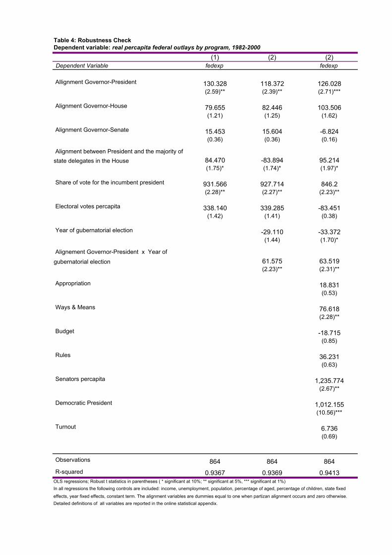
Table 4: Robustness CheckDependent variable: real percapita federal outlays by program, 1982-2000

(1) (2) (2)Dependent Variable fedexp fedexp

Allignment Governor-President 130.328 118.372 126.028(2.59)** (2.39)** (2.71)***

Alignment Governor-House 79.655 82.446 103.506(1.21) (1.25) (1.62)

Alignment Governor-Senate 15.453 15.604 -6.824(0.36) (0.36) (0.16)

Alignment between President and the majority of state delegates in the House 84.470 -83.894 95.214

(1.75)* (1.74)* (1.97)*

Share of vote for the incumbent president 931.566 927.714 846.2(2.28)** (2.27)** (2.23)**

Electoral votes percapita 338.140 339.285 -83.451(1.42) (1.41) (0.38)

Year of gubernatorial election -29.110 -33.372(1.44) (1.70)*

Alignement Governor-President x Year of

gubernatorial election 61.575 63.519(2.23)** (2.31)**

Appropriation 18.831(0.53)

Ways & Means 76.618(2.28)**

Budget -18.715(0.85)

Rules 36.231(0.63)

Senators percapita 1,235.774(2.67)**

Democratic President 1,012.155(10.56)***

Turnout 6.736(0.69)

Observations 864 864 864 R-squared 0.9367 0.9369 0.9413OLS regressions; Robust t statistics in parentheses ( * significant at 10%; ** significant at 5%, *** significant at 1%)In all regressions the following controls are included: income, unemployment, population, percentage of aged, percentage of children, state fixed

effects, year fixed effects, constant term. The alignment variables are dummies equal to one when partizan alignment occurs and zero otherwise.Detailed definitions of all variables are reported in the online statistical appendix.

Statistical Appendix

1 Summary Statistics (Table A1)

Table A1 reports summary statistics of the variables we used in the paper.

2 Multicollinearity (Tables A2-A4)

Most of the explanatory variables used in the regressions could be correlatedand therefore generate large standard errors. It is therefore important to verifywhether the low signi�cance of some variables, and especially of the closenessand swing variables, is due to multicollinearity. For this purpose we use thevariance in�ation factor (Chatterjee, Hadi and Price 2000) which, for a variablexj is given by:

V IF (xj) =1

1�R2jwhere R2j is the square of the multiple correlation coe¢ cient that results whenxj is regressed against all the other explanatory variables.The variance of any bj coe¢ cient in a multiple regression is:

V ar [bj ] =�2�

1�R2j�Sxjxj

where �2 is the square of the random disturbance and Sxjxj is the variance ofthe xj variable. The bigger R2j and therefore V IF (xj) = (

1

(1�R2j)), the greater

is V ar [bj ], for a given level of �2

Sxjxj. An informal rule of thumb applied by most

analysts (Chatterjee, Hadi and Price, 2000) is that a variance in�ation factor inexcess of 20 may be evidence of multicollinearity.In column 1 of table A2 we report the VIF relative to the regressions of

table 2. In column 1 (which refers to column1 of Table 2) the variance in�ationfactor turns out to be 8.78 for the share of the presidential vote and and 7.12 forthe closeness of the last presidential election. This means that the collinearityof these two variables with the other predictors is acceptable and does notsigni�cantly in�ate the estimation of their standard errors. In the second columnof table A2 (which refers to column 2 in Table 2) we obtain a VIF of 2.97 forthe presidential share and of 2.13 for the swing variable. Hence, again, we canexclude that the low signi�cance of the swing variable is due to multicollinearity.The only variable for which we detect a potential multicollinearity problem isthe number of presidential electoral votes per capita with a V IF = 41:02 whichmeans that the standard error of this coe¢ cient is highly in�ated. Therefore, weshould use caution in stating that the coe¢ cient of this variable is not signi�cantas it appears in the regression of column 2. In column 1 the number of electoralvotes per capita is signi�cant at the 10% level, again indicating that one shouldnot underestimate the relevance of such variable.

1

In Table A3 we report the results referred to Table 3 in the paper. In thiscase all variables display a VIF which is well below the threshold we establishedand therefore we can conclude that multicollinerarity is not a problem in thesespeci�cations.Table A4 (which refers to Table 4 in the paper) is potentially the most prob-

lematic, since we include a number of indicators of alignment that are probablycorrelated. However, it appears from the VIFs that multicollinearity should notplay a big role in in�ating the standard errors of such variables. Once again,instead, we �nd that multicollineraity is a problem for the overrepresentationvariables, namely the number of senators per capita and the number of elec-toral votes per capita. In the case of senators per capita this is not su¢ cient torender the estimation insigni�cant (the coe¢ cient is in fact signi�cat at the 5%level). In the case of electoral votes per capita we get an insigni�cant coe¢ cientbut this results should be clearly interpreted with some caution. Nevertheless,overrepresentation represents only a control factor for our regressions and theimportant point is that our variables of interest do not appear to su¤er from amulticollinearity problem.

3 More on the swing-voter hypothesis (Table A5)

In the paper we reach the conclusion that swing states do not receive morefederal funds, while states where the president obtains a larger share of votestend to be rewarded. Our conclusion does not depend on the speci�c measurewe use. In the paper we de�ne a swing state in the following way:

� De�ne swing_last as a dummy equal to 1 if the state swung at the lastpresidential election. Let i = 1; 2; 3; 4 indicate the four previous presiden-tial elections at each given time. Also, t indicates the years and k = 1; :::48indicates a state; then

swing1kt =4Xi=1

swing_lastkt=4 :

In other words, swing1 (indicated in the table as Long term swing 4 yearsaverage) is the average of swing_last over the previous four elections.

In this Appendix we report regressions where two alternative measures havebeen used. In column 1 of Table A5 we report regressions where swing_last hasbeen used instead of swing. In column 2 of table A5 we use instead a variablede�ned as follows:

� Let i = 1; 2; :::N indicate at each given time all previous presidentialelections since 1964. Also, t indicates the years and k = 1; :::48 indicatesa state; then

swing2kt =NXi=1

swing_lastkt=N :

2

In other words, swing2 (indicated in the table as Long term swing since1964) is in this case the average of swing_last over all elections between1964 and t.

The results in table A5 show that such variations make very little di¤erence.Our results are robust to the use of such alternative variables and continueto support the idea that swing states do not have any statistically signi�cantadvantage in terms of the receipt of federal funds.In the column 3 of Table A5 we report an additional speci�cation with

respect to the swing-voter hypothesis. While we show that swing states do notreceive more funds, it is still possible that the direction of the swing matters.In other terms, a greater allocation of funds could be expected for states thatswing in the direction of the president as opposed to states that move awayfrom him. Thus, in column 3 we introduce a dummy variable equal to 1 forstates that swung in the direction of the president in the last election and aninteraction term between this dummy and the swing variable. Both the dummyand the interaction turn out to be statistically insigni�cant. We conclude fromthis analysis that swing states do not receive more federal funds.

3

Table A1: Summary StatisticsVariable Obs Mean Std. Dev Min Max

Federal Expenditure per Capita* 912 5066.518 983.5352 3005.729 8824.92

Alignment Governor-President 960 0.40625 0.4913883 0 1

Alignment Governor-House 960 0.5979167 0.4905742 0 1

Alignment Governor-Senate 960 0.5208333 0.4998262 0 1

Alignment between Governor and the majority of state delegates to House

960 0.421875 0.4941162 0 1

Alignment between Governor and the 960 0.284375 0.4513514 0 1two senators**

Alignment between President and the 960 0.2645833 0.441341 0 1two senators**

Alignment between President and the 960 0.5333333 0.4991477 0 1majority of state delegates to House

Alignment between the majority of state 960 0.5916667 0.4917816 0 1delegates to House and House majority

Alignment between the two senators 960 0.3291667 0.4701555 0 1and the Senate majority

Appropriation 960 1.734375 1.430804 0 8

Ways & Means 960 0.5104167 0.7362899 0 4

Budget 960 0.8104167 1.107137 0 6

Rules 960 0.3177083 0.6161698 0 3

Closeness in Past Presid. Election 960 0.1377484 0.1058159 0.0015169 0.5220283

Share of Votes for President 960 0.5121536 0.0898193 0.2465447 0.7450179

State Elect. Votes per Capita 960 2.714539 1.024855 1.527064 6.616543

Senators per Capita 960 0.9661192 0.9851338 0.0588056 4.411028

Swing 912 0.3723246 0.2042428 0 1

Democratic President 960 0.4 0.4901533 0 1

Gubernatorial election year 960 0.2625 0.4402222 0 1

Turnout 960 61.02875 6.571284 46.1 75.6

Income per Capita* 960 22954.47 4292.623 13796.28 41446.37

Unemployment 960 6.074167 2.200156 2.2 18

Total Population 960 5217.995 5497.381 453.409 34010.38

Share of population aged above 65 960 0.1239534 0.0199277 0.0468377 0.3663689

Share of Population aged 5-17 960 0.1910132 0.0226012 0.0233483 0.6194438

Notes. *Federal Expenditure and Income are expressed in real value (year 2000). **These variables take value equal to 1 when both senators are of the same political colour of, respectively, tthe Governor and the Presiden

Table A2: VIF relative to the coefficients of the regressions in table 2Variable (1) (2)electoral votes per capita 41.91 41.02share of votes for the president 8.76 2.97closeness 7.27swing 2.13

Table A3: VIF relative to the coefficients of the regressions in table 3Variable (1) (2)Alignment Governor-President 3.59 3.69Alignment Governor-House 4.03 4.62Alignment Governor-Senate 1.67 1.75Alignment between the Governor and the 2.03majority of state delegates to the House

Alignment between the Governor and 1.96two state senators

Alignment between the President and the 14.13majority of state delegates in the House

Alignment between the President and the 1.63two state senators

Alignment between the majority of state 13.70delegates in the House and the House majority

Alignment between the two senators of the 1.60State and the Senate majority

Table A4: VIF relative to the coefficients of the regressions in table 4.Variable (1) (2) (3)Alignment Governor-President 3.61 3.84 3.91Alignment Governor-House 4.05 4.06 4.14Alignment Governor-Senate 1.68 1.68 1.73Alignement between the President and a 2.35 2.35 2.54majority of state delegates to the House

Share of votes for the incumbent President 3.27 3.27 3.38Electoral votes per capita 43.98 43.99 112.13Year of gubernatorial election 2.61 2.62Alignement Governor-President x Year of gubernatorial election 2.39 2.40Appropriation 9.46Ways & Means 3.90Budget 3.74Rules 3.79Senators per capita 477.91Democratic President 17.17Turnout 10.19

Table A5: More on Swing BiasDependent variable: real percapita federal outlays, 1982-2000

(1) (2) (3)Dependent Variable fedexp fedexp fedexp

Share of vote for the incumbent president 1154.21 1078.26 1169.77(2.66)** (2.29)** (2.65)**

Long term Swing (4 years) -16.51(0.09)

Swing_last 26.7636(0.57)

Long term Swing (since 1964) -147.04(1.02)

State where the President won -113.55(0.91)

State where the President Won x Long termSwing -140.90

(0.66) Electoral votes percapita 370.24 360.82 302.01

(1.70)* (1.62) (1.41) Observations 864 864 864 R-squared 0.9348 0.9351 0.9369OLS regressions; Robust t statistics in parentheses (* significant at 10%; ** significant at 5%; *** significant at 1%)

In all regressions the following controls are included: income, unemployment, population, percentage of aged, percentage of children,

state fixed effects, year fixed effects, constant term.

Table A6: More on AlignmentsDependent variable: real percapita federal outlays, 1982-2000

(2) (3) (4)Dependent Variable fedexp fedexp fedexp

Alignment between Governor and the majority of state delegates in the House -39.4412

(0.99)Alignment between Governor and the two state

senators -74.9903(1.39)

Alignment between President and the two statesenators 15.6720

(0.27) Alignment between President and the majority of state delegates in the House 175.688

(3.13)*** Alignment between the majority of state delegates in the House and the House majority -154.624

(2.61)** Alignment between the two senators of the state and the Senate majority -5.9300

(0.14)

Observations 864 864 864 R-squared 0.9271 0.9302 0.9292OLS regressions; Robust t statistics in parentheses (* significant at 10%; ** significant at 5%; *** significant at 1%)In all regressions the following controls are included: income, unemployment, population, percentage of aged, percentage of children, state fixedeffects, year fixed effects, constant term. The alignment variables are dummies equal to one when partizan alignment occurs and zero otherwise.Detailed definitions of all variables are reported in the online statistical appendix

List of variables: Definitions and Sources From the Statistical Abstract of the US and the Bureau of Statistics Federal expenditure: real federal expenditure by state (year 2000 constant USD per capita). Income: real income (year 2000 constant USD per capita). Population: state population divided by 1000. Turnout: total percentage of voting population in the last presidential election. Percentage of Aged: share of the population over 65 years old by state. Percentage of Children: share of the population between 5 and 17 years old by state. Unemployment: unemployment rate. Democratic president: dummy variable equal to 1 when the President is democratic, and zero when the President is republican. Governor election year: dummy variable equal to 1 during a governor election year and zero otherwise. Authors’ elaboration on data from the Statistical Abstract of the United States Closeness: distance in the percentage of vote (by state) between the winner of the presidential race and the runner up. Share of vote for the incumbent president: share of votes for the current President in the last presidential elections. Last election swing: dummy equal to 1 if the state swung at the last presidential election. Swing: moving average of “Last election swing” over the four previous presidential elections at each given time. Long term swing: average of “Last election swing” from 1964 to the last election. Alignment Governor-President: dummy variable equal to one when the party affiliation of the governor is the same as that of the President, and zero otherwise. Alignment Governor-House: dummy variable equal to one when the party affiliation of the governor is the same as that of the majority of the House, and zero otherwise. Alignment Governor-Senate: dummy variable equal to one when the party affiliation of the governor is the same as that of the majority of the Senate, and zero otherwise. Senators percapita: 2000/Population. Electoral votes percapita: (1000×Electoral votes)/Population Alignment between the governor and the two state senators: dummy variable equal to one when the governor is from the same party of both senators in the state, and zero otherwise. Alignment between the Governor and the majority of state delegates in the House: dummy variable equal to one when the governor is from the same party as the majority of state delegates in the House, and zero otherwise. Alignment between the President and the two state senators: dummy variable equal to 1 if both senators from a state are of the same party of the President.

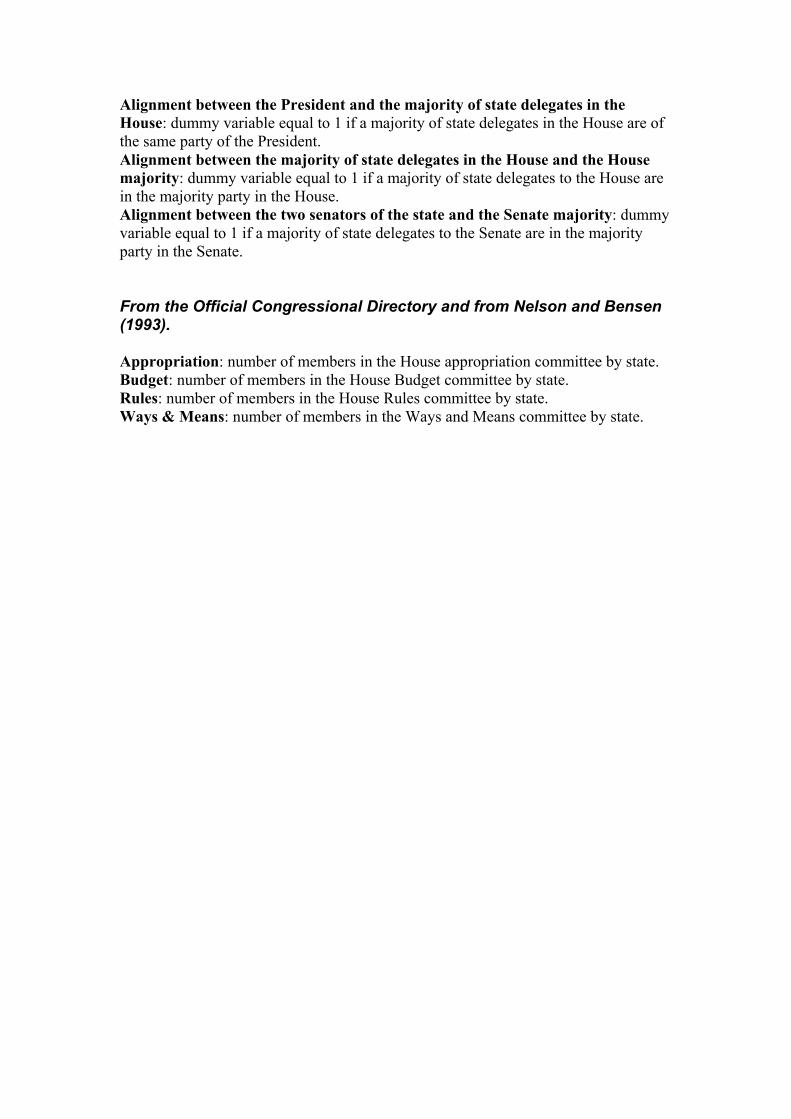
Alignment between the President and the majority of state delegates in the House: dummy variable equal to 1 if a majority of state delegates in the House are of the same party of the President. Alignment between the majority of state delegates in the House and the House majority: dummy variable equal to 1 if a majority of state delegates to the House are in the majority party in the House. Alignment between the two senators of the state and the Senate majority: dummy variable equal to 1 if a majority of state delegates to the Senate are in the majority party in the Senate. From the Official Congressional Directory and from Nelson and Bensen (1993). Appropriation: number of members in the House appropriation committee by state. Budget: number of members in the House Budget committee by state. Rules: number of members in the House Rules committee by state. Ways & Means: number of members in the Ways and Means committee by state.