Algoritmi Genetici
65
Modelli Computazionali per Sistemi Complessi 2003/2004 University of Calabria Genetic Algorithms Dr. Donato D’Ambrosio Dr. William Spataro Prof. Salvatore Di Gregorio
-
Upload
khangminh22 -
Category
Documents
-
view
3 -
download
0
Transcript of Algoritmi Genetici
Modelli Computazionali per Sistemi Complessi2003/2004
University of Calabria
Genetic Algorithms
Dr. Donato D’AmbrosioDr. William Spataro
Prof. Salvatore Di Gregorio
Search Algorithms
• Search Algorithms can be subdivided in two main categories:– Exact (e.g. algorithms in Numerical Analysis)– Heuristic (algorithms based on random search
criteria) • A search problem is called “difficult” (e.g. the
TSP - Traveller Salesman Problem) if does not exist an algorithm that solve it or, if such an algorithm exists, it doesn’t solve the problem in polynomial time
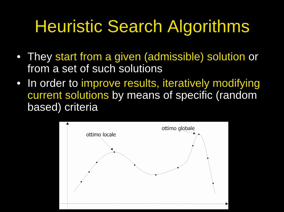
Heuristic Search Algorithms• They start from a given (admissible) solution or
from a set of such solutions• In order to improve results, iteratively modifying
current solutions by means of specific (random based) criteria
What is and how does work a genetic algorithm
• Genetic Algorithms (GAs) were proposed by John Holland (University of Michigan) between the end of the 60s and the beginning of the 70s
• GAs (Holland, 1975, Goldberg, 1989) are search algorithms inspired from the mechanisms of the Darwinian Natural Selection and from Genetics
• GAs simulate the evolution of a population of individuals, representing candidate solutions to a specific search problem, by favoring the surviving and the reproduction of the best
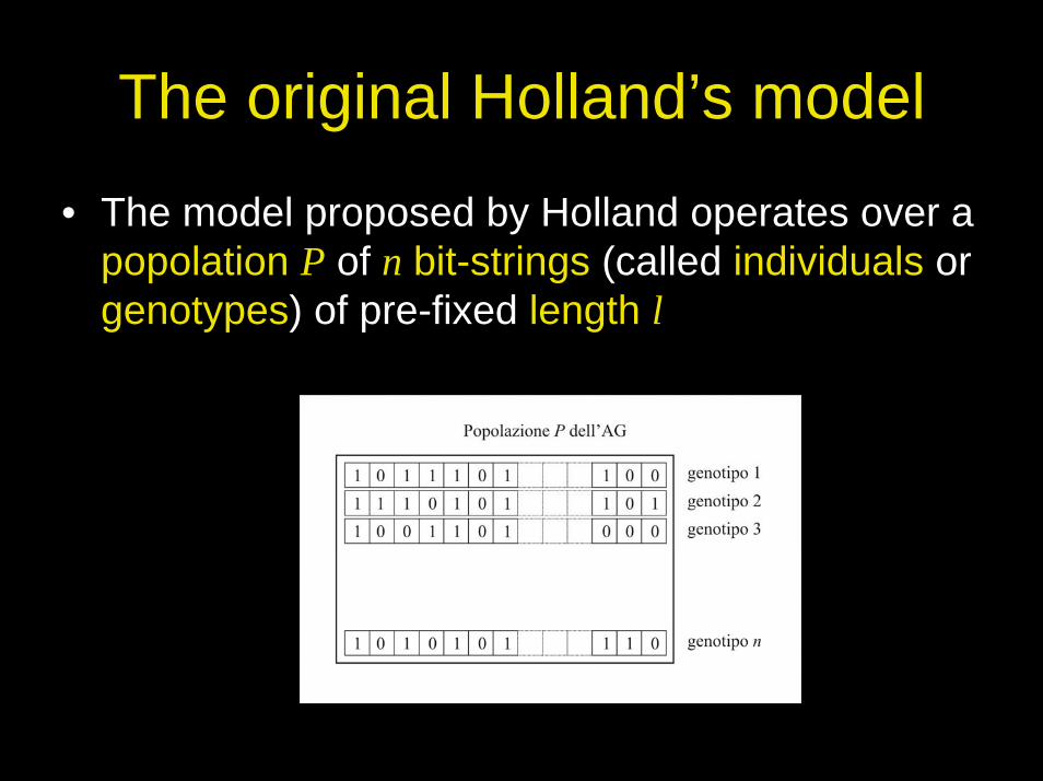
The original Holland’s model
• The model proposed by Holland operates over a popolation P of n bit-strings (called individuals or genotypes) of pre-fixed length l
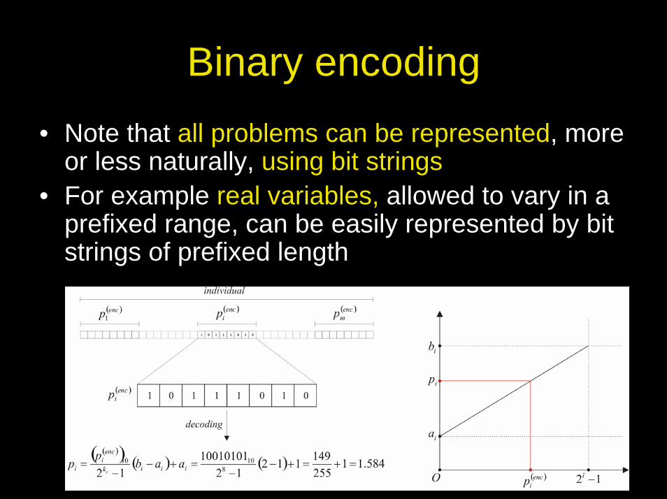
Binary encoding• Note that all problems can be represented, more
or less naturally, using bit strings• For example real variables, allowed to vary in a
prefixed range, can be easily represented by bit strings of prefixed length
Fitness function, search space and fitness landscape
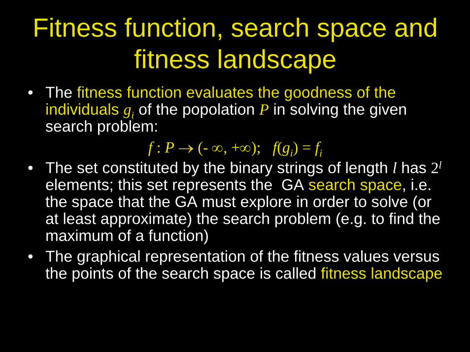
• The fitness function evaluates the goodness of the individuals gi of the popolation P in solving the given search problem:
f : P → (- ∞, +∞); f(gi) = fi• The set constituted by the binary strings of length l has 2l
elements; this set represents the GA search space, i.e. the space that the GA must explore in order to solve (or at least approximate) the search problem (e.g. to find the maximum of a function)
• The graphical representation of the fitness values versus the points of the search space is called fitness landscape
Example of fitness landscape for a binary GA
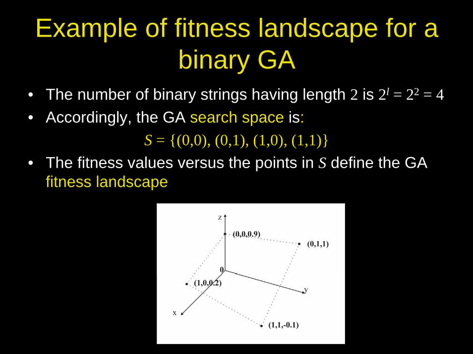
• The number of binary strings having length 2 is 2l = 22 = 4• Accordingly, the GA search space is:
S = {(0,0), (0,1), (1,0), (1,1)}• The fitness values versus the points in S define the GA
fitness landscape
Operators• Once the fitness function has determined the
goodness of each individual, a new population of individuals (or genotypes) is created by applying many operators inspired from Natural Selection and Genetics
• The operators proposed by Holland are:– Selection (inspired to Natural Selection)– Crossover (inspired to Genetics)– Mutation (inspired to Genetics)
• Crossover and Mutation are called geneticoperators
The selection Operator
• The Darwinian Natural Selection asserts that the stronger individuals have higher probability to survive inside their living environment, thus higher probability to reproduce their selves
• In the Holland GA context, stronger individuals correspond to those having higher fitness, as they better solve the given search problem; as a consequence, they must be privileged during the selection of the individuals that will undergo reproduction to form new individuals
The proportional selection
• Holland suggested a selection method proportional to the individuals’ fitness
• let fi the fitness of the genotype gi, then the probability that gi is selected for the reproduction is:
ps,i = fi / Σfj
• Such probabilities are used to construct a kind of probability’s roulette
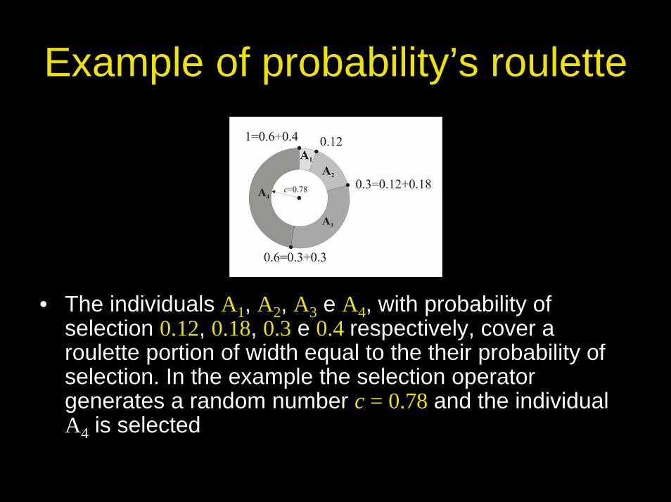
Example of probability’s roulette
• The individuals A1, A2, A3 e A4, with probability of selection 0.12, 0.18, 0.3 e 0.4 respectively, cover a roulette portion of width equal to the their probability of selection. In the example the selection operator generates a random number c = 0.78 and the individual A4 is selected
Mating pool• Each time that an individual is selected, a
perfect copy is created and inserted in the so-called mating pool
• Once that the mating pool is filled with exactly ncopies of individuals of the GA population (where n is the population size), a new set of noffspring are generated by applying the genetic operators (i.e. crossover and mutation)
• A selection operator that replaces all the population with new individuals, as the one proposed by Holland, is called generational
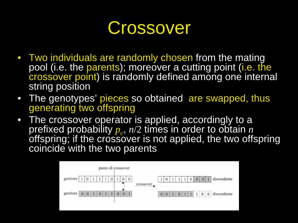
Crossover• Two individuals are randomly chosen from the mating
pool (i.e. the parents); moreover a cutting point (i.e. the crossover point) is randomly defined among one internal string position
• The genotypes’ pieces so obtained are swapped, thus generating two offspring
• The crossover operator is applied, accordingly to a prefixed probability pc, n/2 times in order to obtain noffspring; if the crossover is not applied, the two offspring coincide with the two parents
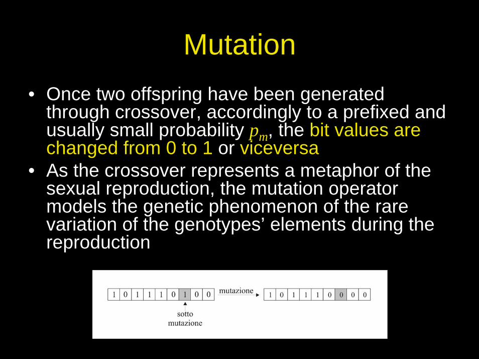
Mutation• Once two offspring have been generated
through crossover, accordingly to a prefixed and usually small probability pm, the bit values are changed from 0 to 1 or viceversa
• As the crossover represents a metaphor of the sexual reproduction, the mutation operator models the genetic phenomenon of the rare variation of the genotypes’ elements during the reproduction
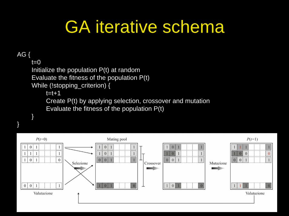
GA iterative schemaAG {
t=0Initialize the population P(t) at randomEvaluate the fitness of the population P(t)While (!stopping_criterion) {
t=t+1Create P(t) by applying selection, crossover and mutationEvaluate the fitness of the population P(t)
}}
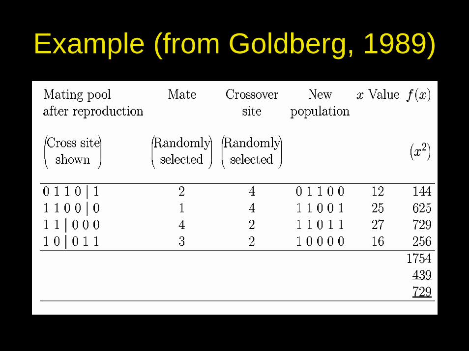
Example (from Goldberg, 1989)• Search (easy!) problem: find the maximum of the
function y=x2 in the range [0,31]• GA approach:
– Genotypes’ representation: binary strings (e.g. 00000↔0; 01101↔13; 11111↔31)
– Population size: 4– Crossover and no mutation (just an example!)– Roulette wheel selection (i.e. the proportional one)– Random initialization
• One generational cycle with the hand shown
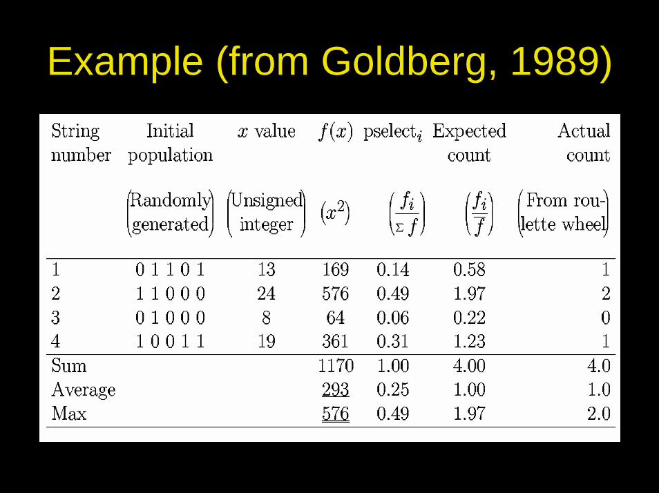
Example (from Goldberg, 1989)
Example (from Goldberg, 1989)
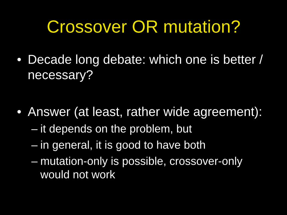
Crossover OR mutation?
• Decade long debate: which one is better / necessary?
• Answer (at least, rather wide agreement):– it depends on the problem, but– in general, it is good to have both– mutation-only is possible, crossover-only
would not work
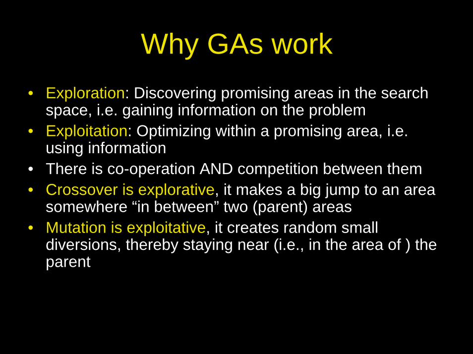
Why GAs work• Exploration: Discovering promising areas in the search
space, i.e. gaining information on the problem• Exploitation: Optimizing within a promising area, i.e.
using information• There is co-operation AND competition between them• Crossover is explorative, it makes a big jump to an area
somewhere “in between” two (parent) areas• Mutation is exploitative, it creates random small
diversions, thereby staying near (i.e., in the area of ) the parent
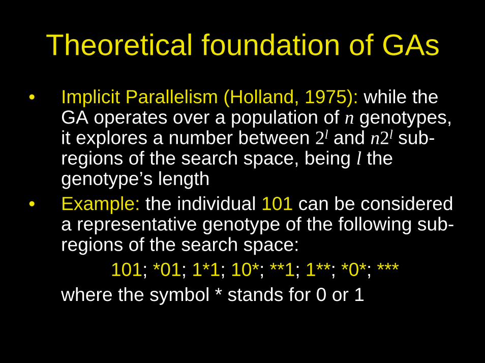
Theoretical foundation of GAs• Implicit Parallelism (Holland, 1975): while the
GA operates over a population of n genotypes, it explores a number between 2l and n2l sub-regions of the search space, being l the genotype’s length
• Example: the individual 101 can be considered a representative genotype of the following sub-regions of the search space:
101; *01; 1*1; 10*; **1; 1**; *0*; ***where the symbol * stands for 0 or 1
Theoretical foundation of GAs
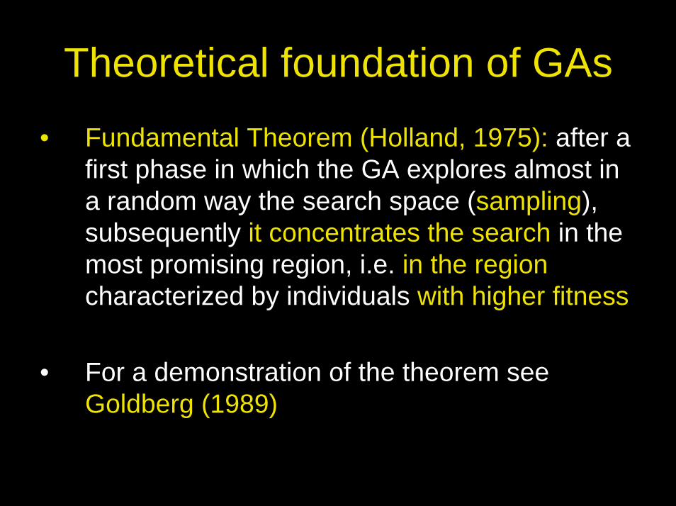
• Fundamental Theorem (Holland, 1975): after a first phase in which the GA explores almost in a random way the search space (sampling), subsequently it concentrates the search in the most promising region, i.e. in the regioncharacterized by individuals with higher fitness
• For a demonstration of the theorem see Goldberg (1989)
Other GA models (Encoding)
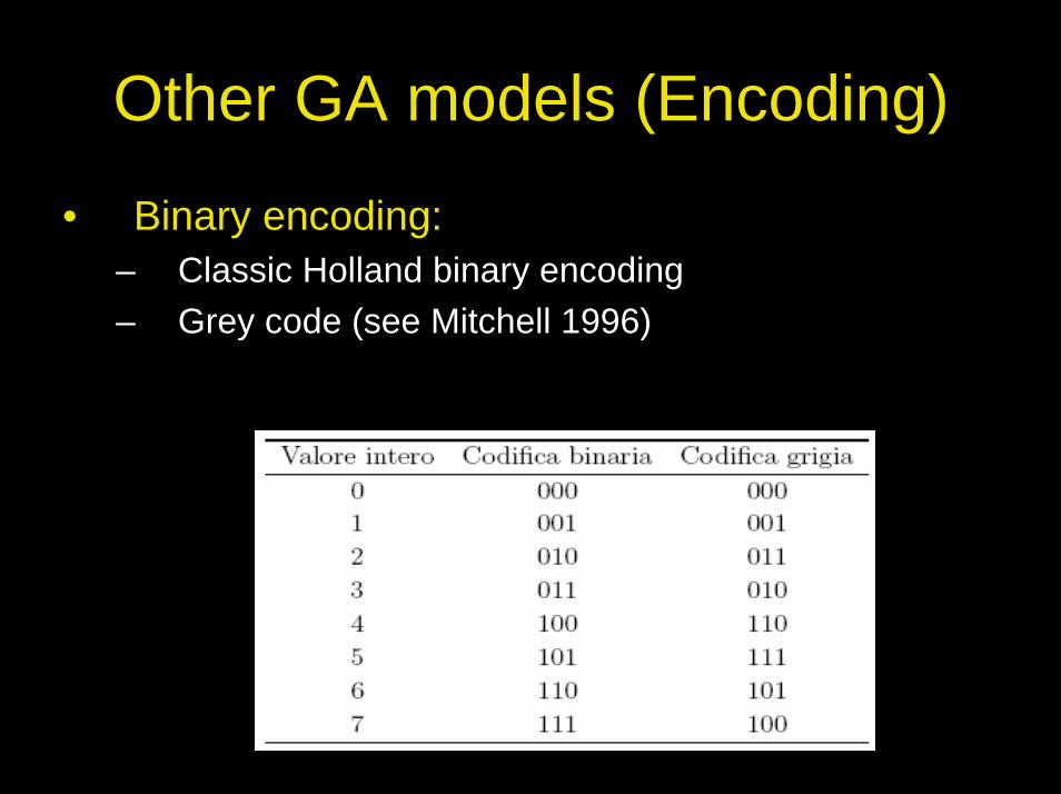
• Binary encoding:– Classic Holland binary encoding – Grey code (see Mitchell 1996)
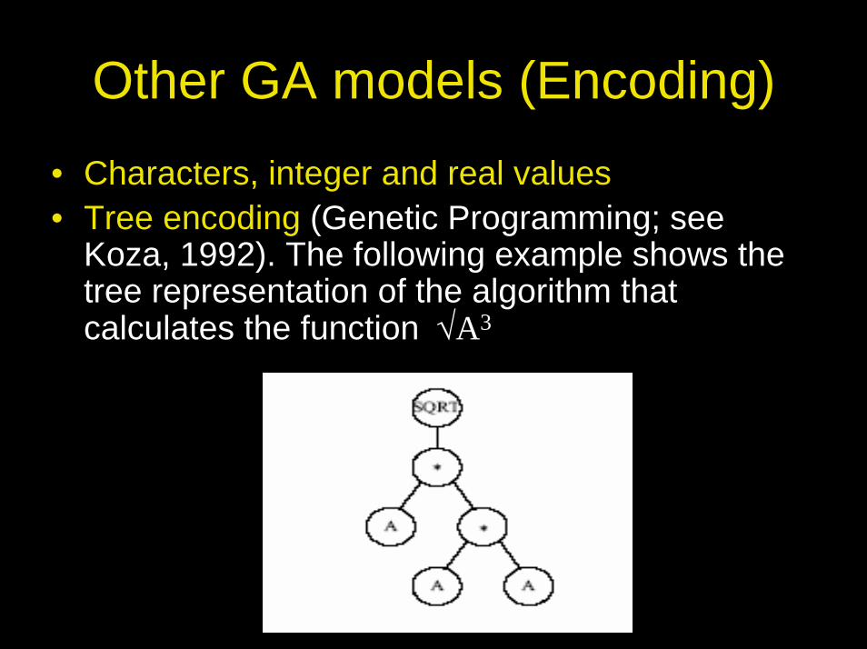
Other GA models (Encoding)• Characters, integer and real values• Tree encoding (Genetic Programming; see
Koza, 1992). The following example shows the tree representation of the algorithm thatcalculates the function √A3
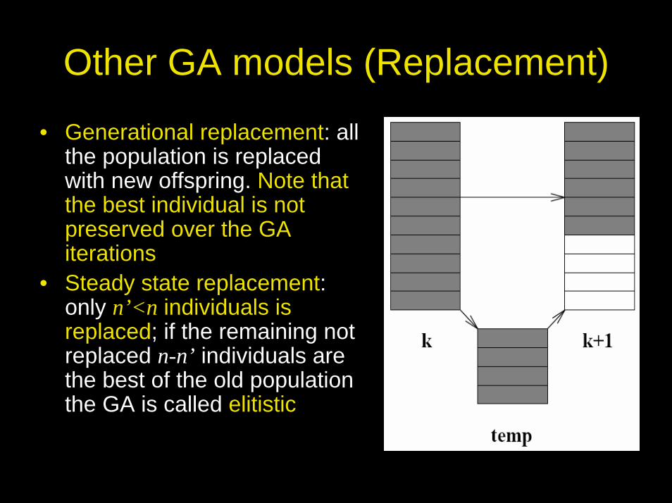
Other GA models (Replacement)
• Generational replacement: all the population is replaced with new offspring. Note that the best individual is not preserved over the GA iterations
• Steady state replacement: only n’<n individuals is replaced; if the remaining not replaced n-n’ individuals are the best of the old population the GA is called elitistic
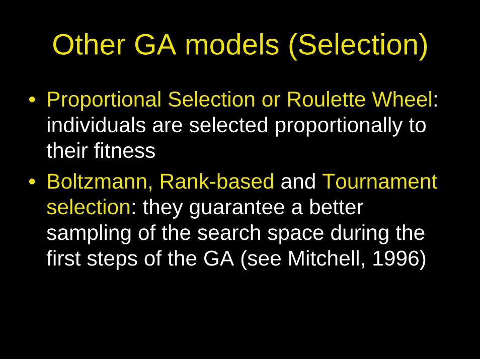
Other GA models (Selection)
• Proportional Selection or Roulette Wheel: individuals are selected proportionally to their fitness
• Boltzmann, Rank-based and Tournament selection: they guarantee a better sampling of the search space during the first steps of the GA (see Mitchell, 1996)
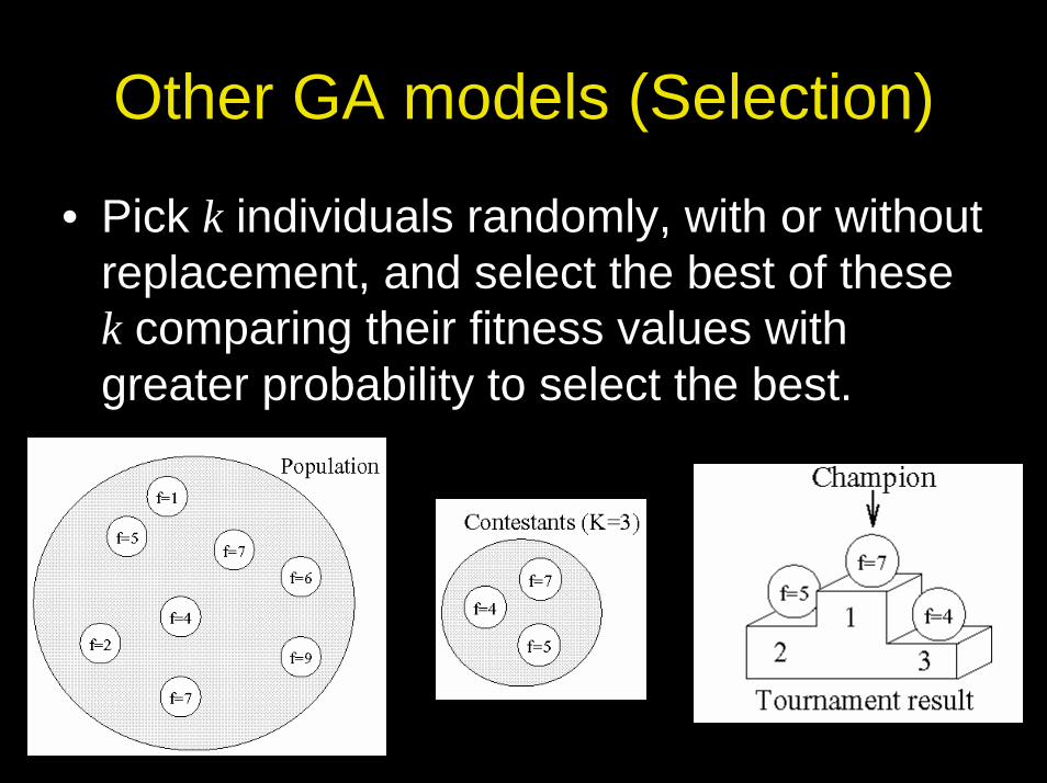
Other GA models (Selection)
• Pick k individuals randomly, with or without replacement, and select the best of these k comparing their fitness values with greater probability to select the best.
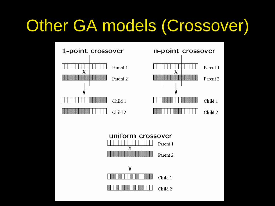
Other GA models (Crossover)
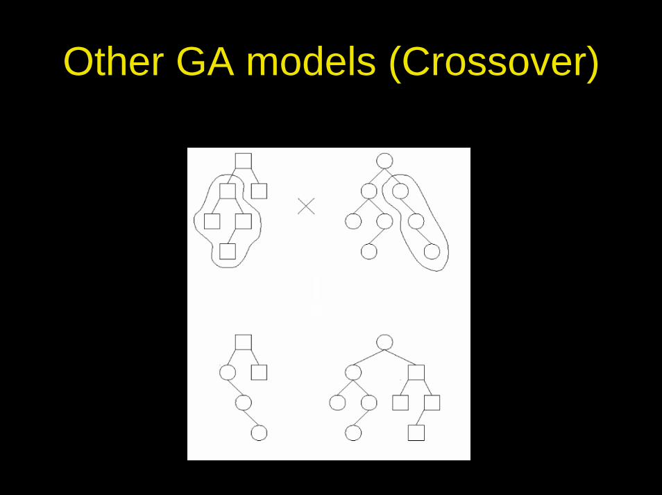
Other GA models (Crossover)
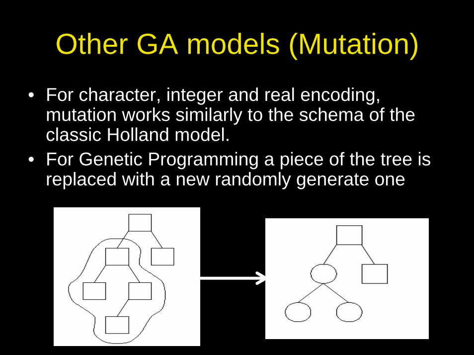
Other GA models (Mutation)• For character, integer and real encoding,
mutation works similarly to the schema of the classic Holland model.
• For Genetic Programming a piece of the tree is replaced with a new randomly generate one
Example• Find the maximum of the function y=x2 in the
range [0,216-1]
1. Chose the size (n) of the population P2. Chose the genotype’s length (l)3. Chose the selection and replacement schema 4. Define a fitness function (f)5. Chose crossover type and fix the probability pc6. Chose mutation type and fix the probability pm 7. Write a program that implements the GA or (better!)
use a free open source GA library
PGAPack• PGAPack is an open source GA library freely
available at the url http://www-fp.mcs.anl.gov/CCST/research/reports_pre1998/comp_bio/stalk/pgapack.html
– It Implements the Holland GA model and many other models successively proposed
– It runs over many operating systems as different UNIX versions and GNU-Linux
– It also Implements a parallel GA model: the Master-Slave GA, thus exploiting (almost transparently for the end user) more CPUs at the same time
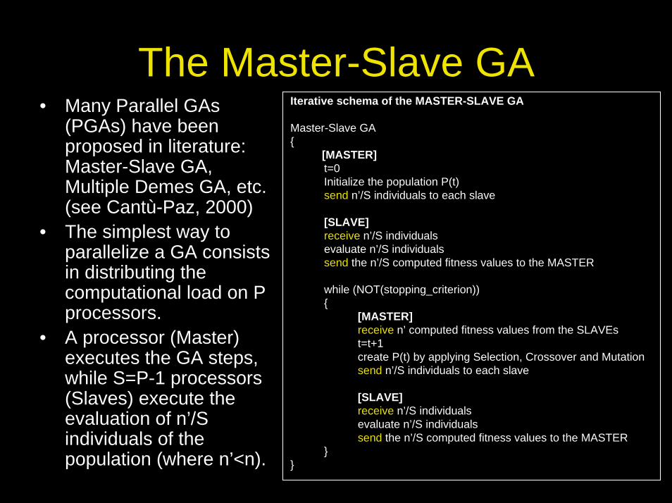
The Master-Slave GAIterative schema of the MASTER-SLAVE GA
Master-Slave GA{
[MASTER]t=0Initialize the population P(t)send n’/S individuals to each slave
[SLAVE]receive n’/S individualsevaluate n’/S individualssend the n’/S computed fitness values to the MASTER
while (NOT(stopping_criterion)){
[MASTER] receive n’ computed fitness values from the SLAVEst=t+1create P(t) by applying Selection, Crossover and Mutationsend n’/S individuals to each slave
[SLAVE]receive n’/S individuals evaluate n’/S individualssend the n’/S computed fitness values to the MASTER
}}
• Many Parallel GAs(PGAs) have been proposed in literature: Master-Slave GA, Multiple Demes GA, etc. (see Cantù-Paz, 2000)
• The simplest way to parallelize a GA consists in distributing the computational load on P processors.
• A processor (Master) executes the GA steps, while S=P-1 processors (Slaves) execute the evaluation of n’/S individuals of the population (where n’<n).
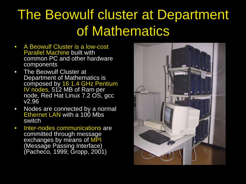
The Beowulf cluster at Department of Mathematics
• A Beowulf Cluster is a low-cost Parallel Machine built with common PC and other hardware components
• The Beowulf Cluster at Department of Mathematics is composed by 16 1.4 GHz Pentium IV nodes, 512 MB of Ram per node, Red Hat Linux 7.2 OS, gccv2.96
• Nodes are connected by a normal Ethernet LAN with a 100 Mbsswitch
• Inter-nodes communications are committed through message exchanges by means of MPI (Message Passing Interface) (Pacheco, 1999; Gropp, 2001)
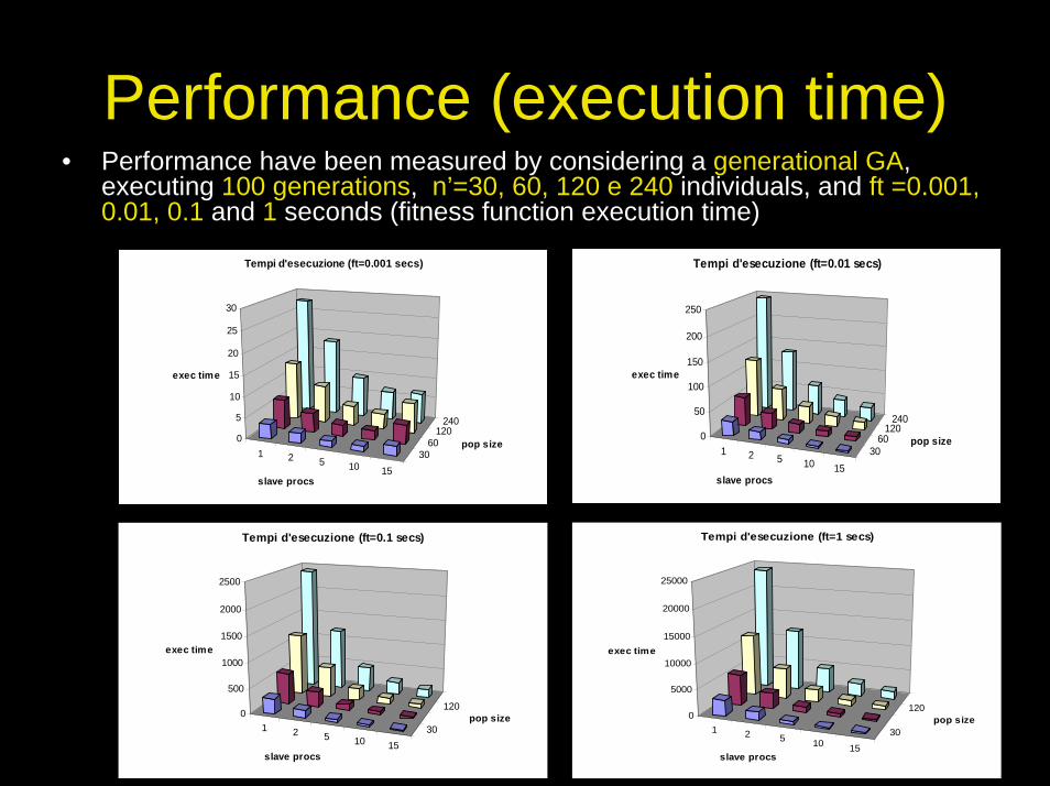
Performance (execution time)• Performance have been measured by considering a generational GA,
executing 100 generations, n’=30, 60, 120 e 240 individuals, and ft =0.001, 0.01, 0.1 and 1 seconds (fitness function execution time)
1 2 5 10 1530
60120
2400
50
100
150
200
250
exec time
slave procs
pop size
Tempi d'esecuzione (ft=0.01 secs)
1 2 5 10 1530
60120
240
0
5
10
15
20
25
30
exec time
slave procs
pop size
Tempi d'esecuzione (ft=0.001 secs)
1 2 5 10 15
30
1200
5000
10000
15000
20000
25000
exec time
slave procs
pop size
Tempi d'esecuzione (ft=1 secs)
1 2 5 10 1530
1200
500
1000
1500
2000
2500
exec time
slave procs
pop size
Tempi d'esecuzione (ft=0.1 secs)
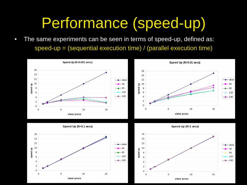
Performance (speed-up)• The same experiments can be seen in terms of speed-up, defined as:
speed-up = (sequential execution time) / (parallel execution time)
Speed Up (ft=0.001 secs)
0
2
4
6
8
10
12
14
16
0 5 10 15
slave procs
spee
d up
ideal
30
60
120
240
Speed Up (ft=0.01 secs)
0
2
4
68
10
12
14
16
0 5 10 15
slave procs
spee
d up
ideal
30
60
120
240
Speed Up (ft=0.1 secs)
0
2
4
6
8
10
12
14
16
0 5 10 15
slave procs
spee
d up
ideal
30
60
120
240
Speed Up (ft=1 secs)
0
2
4
6
8
10
12
14
16
0 5 10 15
slave procs
spee
d up
ideal
30
60
120
240
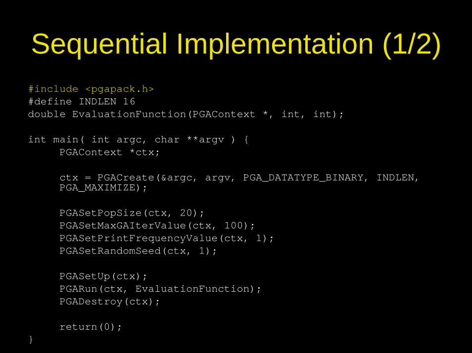
Sequential Implementation (1/2)#include <pgapack.h>#define INDLEN 16double EvaluationFunction(PGAContext *, int, int);
int main( int argc, char **argv ) {PGAContext *ctx;
ctx = PGACreate(&argc, argv, PGA_DATATYPE_BINARY, INDLEN, PGA_MAXIMIZE);
PGASetPopSize(ctx, 20);PGASetMaxGAIterValue(ctx, 100);PGASetPrintFrequencyValue(ctx, 1);PGASetRandomSeed(ctx, 1);
PGASetUp(ctx);PGARun(ctx, EvaluationFunction);PGADestroy(ctx);
return(0);}
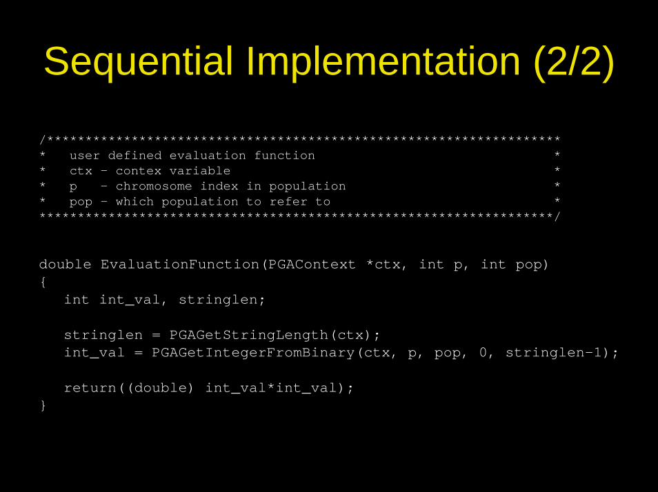
Sequential Implementation (2/2)
/******************************************************************** user defined evaluation function ** ctx - contex variable ** p - chromosome index in population ** pop - which population to refer to ********************************************************************/
double EvaluationFunction(PGAContext *ctx, int p, int pop) {
int int_val, stringlen;
stringlen = PGAGetStringLength(ctx);int_val = PGAGetIntegerFromBinary(ctx, p, pop, 0, stringlen-1);
return((double) int_val*int_val);}
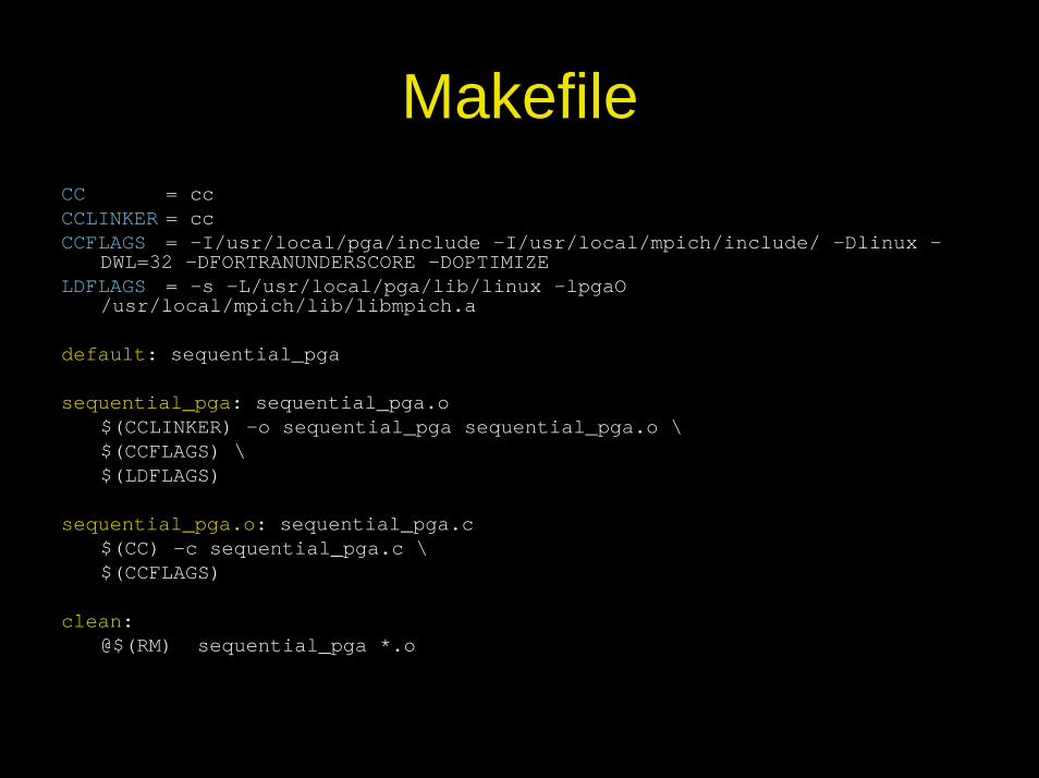
MakefileCC = ccCCLINKER = ccCCFLAGS = -I/usr/local/pga/include -I/usr/local/mpich/include/ -Dlinux -
DWL=32 -DFORTRANUNDERSCORE -DOPTIMIZE LDFLAGS = -s -L/usr/local/pga/lib/linux -lpgaO
/usr/local/mpich/lib/libmpich.a
default: sequential_pga
sequential_pga: sequential_pga.o$(CCLINKER) -o sequential_pga sequential_pga.o \$(CCFLAGS) \$(LDFLAGS)
sequential_pga.o: sequential_pga.c$(CC) -c sequential_pga.c \$(CCFLAGS)
clean: @$(RM) sequential_pga *.o
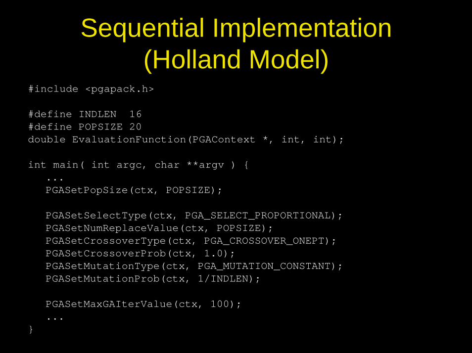
Sequential Implementation (Holland Model)
#include <pgapack.h>
#define INDLEN 16#define POPSIZE 20double EvaluationFunction(PGAContext *, int, int);
int main( int argc, char **argv ) {...PGASetPopSize(ctx, POPSIZE);
PGASetSelectType(ctx, PGA_SELECT_PROPORTIONAL);PGASetNumReplaceValue(ctx, POPSIZE);PGASetCrossoverType(ctx, PGA_CROSSOVER_ONEPT);PGASetCrossoverProb(ctx, 1.0);PGASetMutationType(ctx, PGA_MUTATION_CONSTANT);PGASetMutationProb(ctx, 1/INDLEN);
PGASetMaxGAIterValue(ctx, 100);...
}
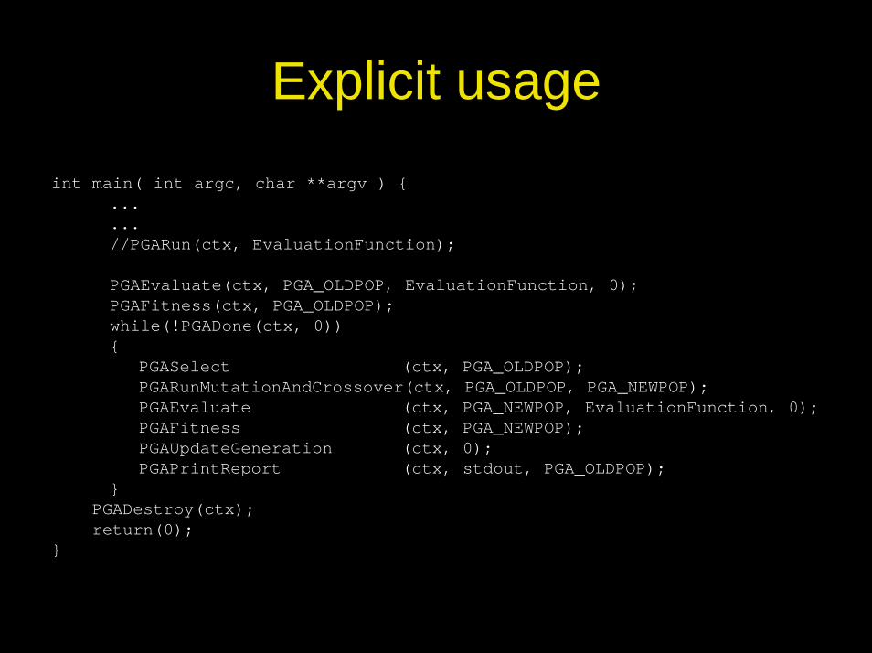
Explicit usage
int main( int argc, char **argv ) {......//PGARun(ctx, EvaluationFunction);
PGAEvaluate(ctx, PGA_OLDPOP, EvaluationFunction, 0);PGAFitness(ctx, PGA_OLDPOP);while(!PGADone(ctx, 0)){
PGASelect (ctx, PGA_OLDPOP);PGARunMutationAndCrossover(ctx, PGA_OLDPOP, PGA_NEWPOP);PGAEvaluate (ctx, PGA_NEWPOP, EvaluationFunction, 0);PGAFitness (ctx, PGA_NEWPOP);PGAUpdateGeneration (ctx, 0);PGAPrintReport (ctx, stdout, PGA_OLDPOP);
}PGADestroy(ctx); return(0);
}
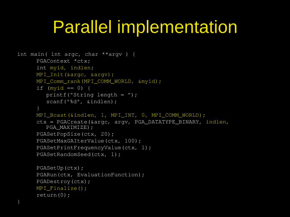
Parallel implementationint main( int argc, char **argv ) {
PGAContext *ctx;int myid, indlen;MPI_Init(&argc, &argv);MPI_Comm_rank(MPI_COMM_WORLD, &myid);if (myid == 0) {
printf("String length = ");scanf("%d", &indlen);
}MPI_Bcast(&indlen, 1, MPI_INT, 0, MPI_COMM_WORLD);ctx = PGACreate(&argc, argv, PGA_DATATYPE_BINARY, indlen,
PGA_MAXIMIZE);PGASetPopSize(ctx, 20);PGASetMaxGAIterValue(ctx, 100);PGASetPrintFrequencyValue(ctx, 1);PGASetRandomSeed(ctx, 1);
PGASetUp(ctx);PGARun(ctx, EvaluationFunction);PGADestroy(ctx);MPI_Finalize();return(0);
}
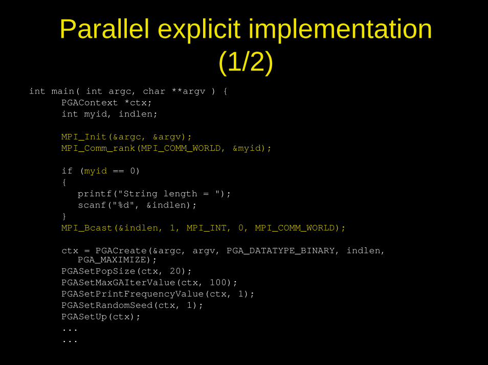
Parallel explicit implementation (1/2)
int main( int argc, char **argv ) {PGAContext *ctx;int myid, indlen;
MPI_Init(&argc, &argv);MPI_Comm_rank(MPI_COMM_WORLD, &myid);
if (myid == 0){
printf("String length = ");scanf("%d", &indlen);
}MPI_Bcast(&indlen, 1, MPI_INT, 0, MPI_COMM_WORLD);
ctx = PGACreate(&argc, argv, PGA_DATATYPE_BINARY, indlen, PGA_MAXIMIZE);
PGASetPopSize(ctx, 20);PGASetMaxGAIterValue(ctx, 100);PGASetPrintFrequencyValue(ctx, 1);PGASetRandomSeed(ctx, 1);PGASetUp(ctx);......
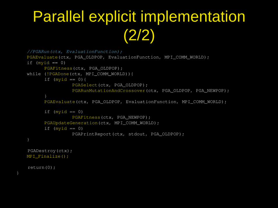
Parallel explicit implementation (2/2)
//PGARun(ctx, EvaluationFunction);PGAEvaluate(ctx, PGA_OLDPOP, EvaluationFunction, MPI_COMM_WORLD);if (myid == 0)
PGAFitness(ctx, PGA_OLDPOP);while (!PGADone(ctx, MPI_COMM_WORLD)){
if (myid == 0){PGASelect(ctx, PGA_OLDPOP);PGARunMutationAndCrossover(ctx, PGA_OLDPOP, PGA_NEWPOP);
}PGAEvaluate(ctx, PGA_OLDPOP, EvaluationFunction, MPI_COMM_WORLD);
if (myid == 0)PGAFitness(ctx, PGA_NEWPOP);
PGAUpdateGeneration(ctx, MPI_COMM_WORLD);if (myid == 0)
PGAPrintReport(ctx, stdout, PGA_OLDPOP);}
PGADestroy(ctx); MPI_Finalize();
return(0);}
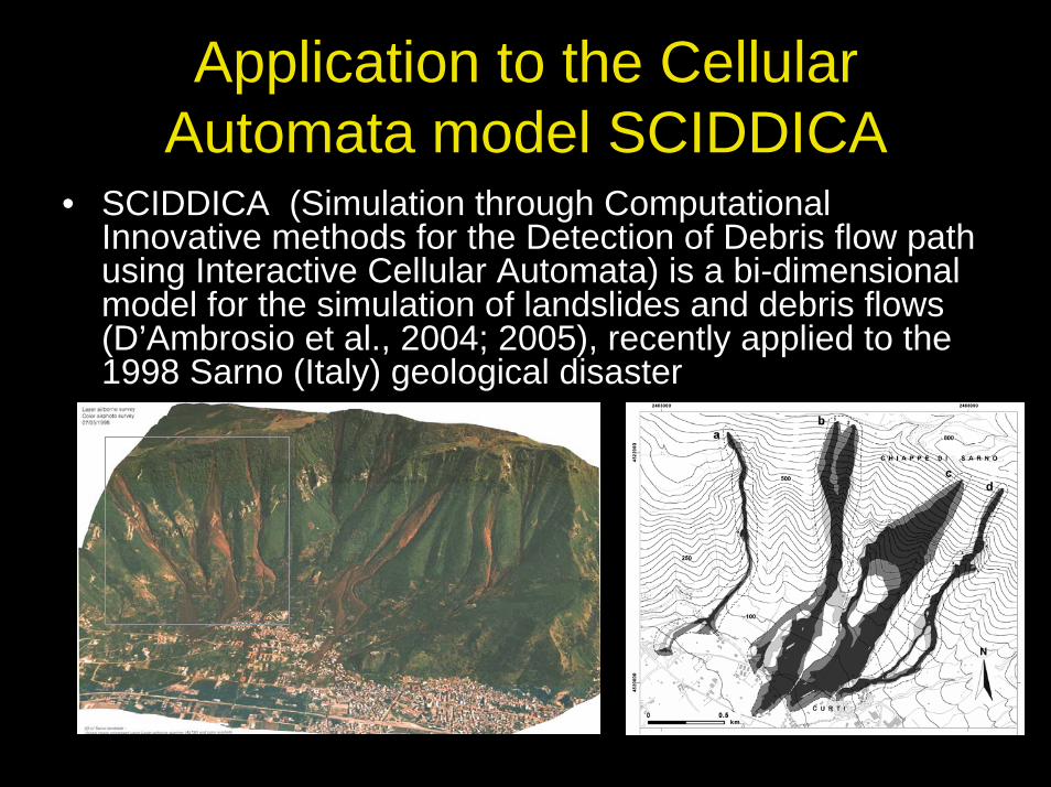
Application to the Cellular Automata model SCIDDICA
• SCIDDICA (Simulation through Computational Innovative methods for the Detection of Debris flow path using Interactive Cellular Automata) is a bi-dimensional model for the simulation of landslides and debris flows (D’Ambrosio et al., 2004; 2005), recently applied to the 1998 Sarno (Italy) geological disaster
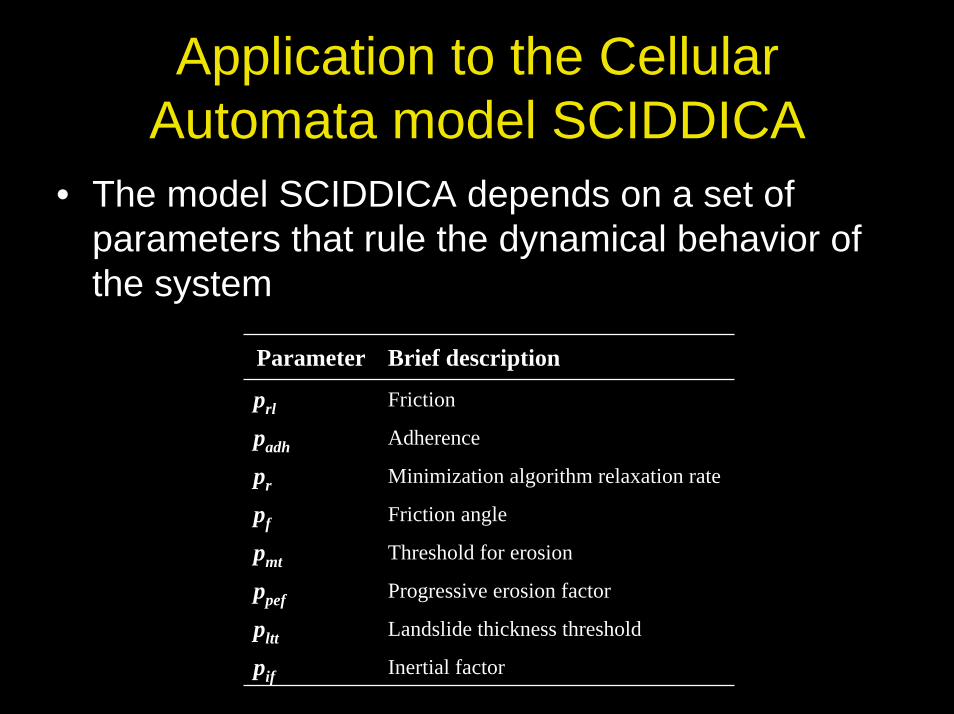
Application to the Cellular Automata model SCIDDICA
• The model SCIDDICA depends on a set of parameters that rule the dynamical behavior of the system
Parameter Brief description
prl Friction
padh Adherence
pr Minimization algorithm relaxation rate
pf Friction angle
pmt Threshold for erosion
ppef Progressive erosion factor
pltt Landslide thickness threshold
pif Inertial factor
Application to the Cellular Automata model SCIDDICA
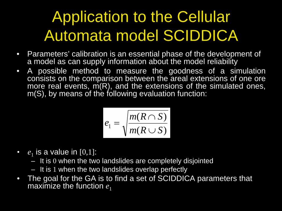
• Parameters’ calibration is an essential phase of the development of a model as can supply information about the model reliability
• A possible method to measure the goodness of a simulation consists on the comparison between the areal extensions of one ore more real events, m(R), and the extensions of the simulated ones, m(S), by means of the following evaluation function:
)()(
1 SRmSRme
∪∩
=
• e1 is a value in [0,1]:– It is 0 when the two landslides are completely disjointed– It is 1 when the two landslides overlap perfectly
• The goal for the GA is to find a set of SCIDDICA parameters thatmaximize the function e1
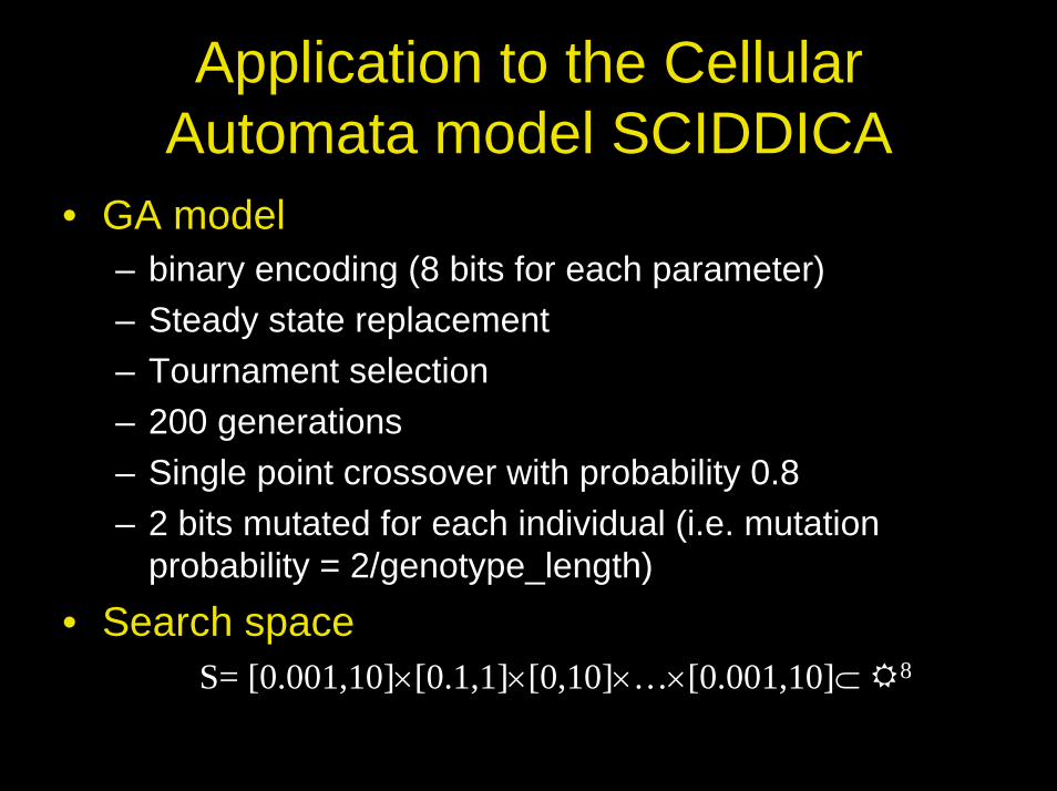
Application to the Cellular Automata model SCIDDICA
• GA model– binary encoding (8 bits for each parameter)– Steady state replacement– Tournament selection– 200 generations– Single point crossover with probability 0.8– 2 bits mutated for each individual (i.e. mutation
probability = 2/genotype_length)• Search space
S= [0.001,10]×[0.1,1]×[0,10]×…×[0.001,10]⊂ 8
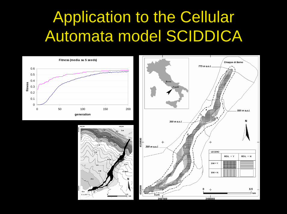
Application to the Cellular Automata model SCIDDICA
Fitness (media su 5 seeds)
0
0.1
0.2
0.3
0.4
0.5
0.6
0 50 100 150 200
generation
fitne
ss
Application to the Cellular Automata model SCIDDICA
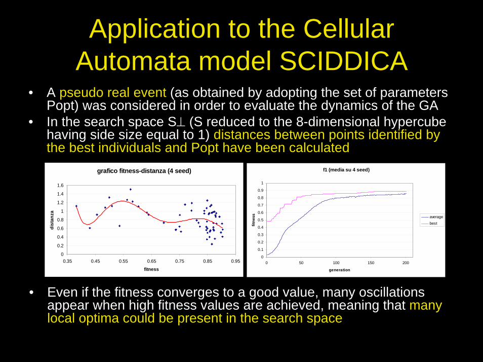
• A pseudo real event (as obtained by adopting the set of parameters Popt) was considered in order to evaluate the dynamics of the GA
• In the search space S⊥ (S reduced to the 8-dimensional hypercube having side size equal to 1) distances between points identified by the best individuals and Popt have been calculated
f1 (media su 4 seed)
0
0.1
0.2
0.3
0.4
0.5
0.6
0.7
0.8
0.9
1
0 50 100 150 200
generation
fitne
ss averagebest
grafico fitness-distanza (4 seed)
0
0.2
0.4
0.6
0.8
1
1.2
1.4
1.6
0.35 0.45 0.55 0.65 0.75 0.85 0.95
fitness
dist
anza
• Even if the fitness converges to a good value, many oscillationsappear when high fitness values are achieved, meaning that many local optima could be present in the search space
Application to the Cellular Automata model SCIDDICA
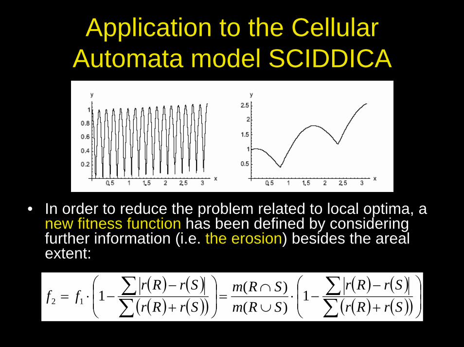
• In order to reduce the problem related to local optima, a new fitness function has been defined by considering further information (i.e. the erosion) besides the arealextent:
( ) ( )( ) ( )( )
( ) ( )( ) ( )( )⎟
⎟⎠
⎞⎜⎜⎝
⎛
+−
−⋅∪∩
=⎟⎟⎠
⎞⎜⎜⎝
⎛
+−
−⋅=∑∑
∑∑
SrRrSrRr
SRmSRm
SrRrSrRr
ff 1)()(112
Application to the Cellular Automata model SCIDDICA
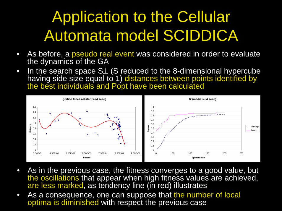
• As before, a pseudo real event was considered in order to evaluate the dynamics of the GA
• In the search space S⊥ (S reduced to the 8-dimensional hypercube having side size equal to 1) distances between points identified by the best individuals and Popt have been calculated
grafico fitness-distanza (4 seed)
0
0.2
0.4
0.6
0.8
1
1.2
1.4
1.6
3.50E-01 4.50E-01 5.50E-01 6.50E-01 7.50E-01 8.50E-01 9.50E-01
fitness
dist
anza
f2 (media su 4 seed)
0
0.1
0.2
0.3
0.4
0.5
0.6
0.7
0.8
0.9
1
0 50 100 150 200 250
generation
fitne
ss averagebest
• As in the previous case, the fitness converges to a good value, but the oscillations that appear when high fitness values are achieved, are less marked, as tendency line (in red) illustrates
• As a consequence, one can suppose that the number of local optima is diminished with respect the previous case
Application to the Cellular Automata model SCIARA
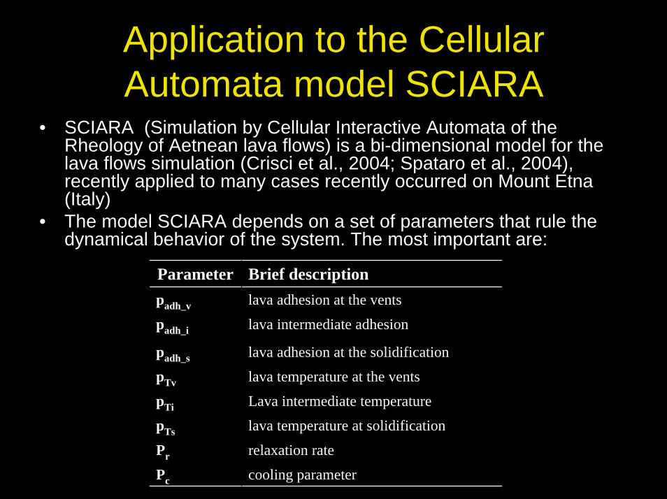
• SCIARA (Simulation by Cellular Interactive Automata of the Rheology of Aetnean lava flows) is a bi-dimensional model for the lava flows simulation (Crisci et al., 2004; Spataro et al., 2004), recently applied to many cases recently occurred on Mount Etna (Italy)
• The model SCIARA depends on a set of parameters that rule the dynamical behavior of the system. The most important are:
Parameter Brief descriptionpadh_v lava adhesion at the vents
padh_i lava intermediate adhesion
padh_s lava adhesion at the solidification
pTv lava temperature at the vents
pTi Lava intermediate temperature
pTs lava temperature at solidification
Pr relaxation rate
Pc cooling parameter
Application to the Cellular Automata model SCIARA
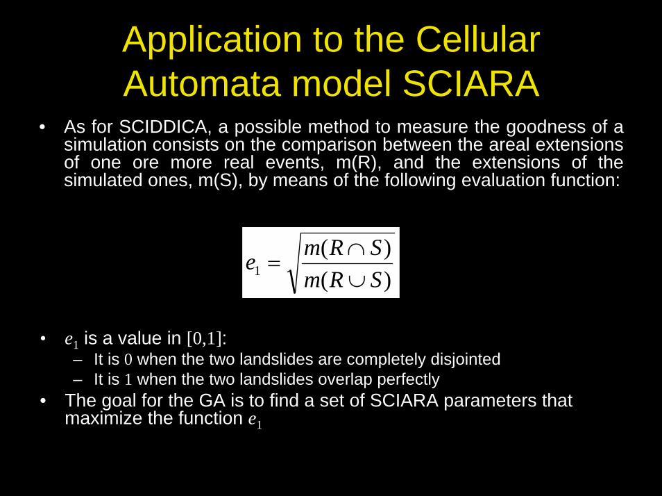
• As for SCIDDICA, a possible method to measure the goodness of a simulation consists on the comparison between the areal extensions of one ore more real events, m(R), and the extensions of the simulated ones, m(S), by means of the following evaluation function:
)()(
1 SRmSRme
∪∩
=
• e1 is a value in [0,1]:– It is 0 when the two landslides are completely disjointed– It is 1 when the two landslides overlap perfectly
• The goal for the GA is to find a set of SCIARA parameters that maximize the function e1
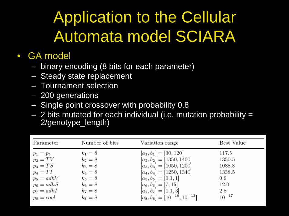
Application to the Cellular Automata model SCIARA
• GA model– binary encoding (8 bits for each parameter)– Steady state replacement– Tournament selection– 200 generations– Single point crossover with probability 0.8– 2 bits mutated for each individual (i.e. mutation probability =
2/genotype_length)
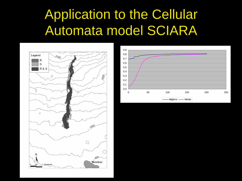
Application to the Cellular Automata model SCIARA
0,0
0,1
0,2
0,3
0,4
0,5
0,6
0,7
0,8
0,9
0 50 100 150 200 250
Migliore Media
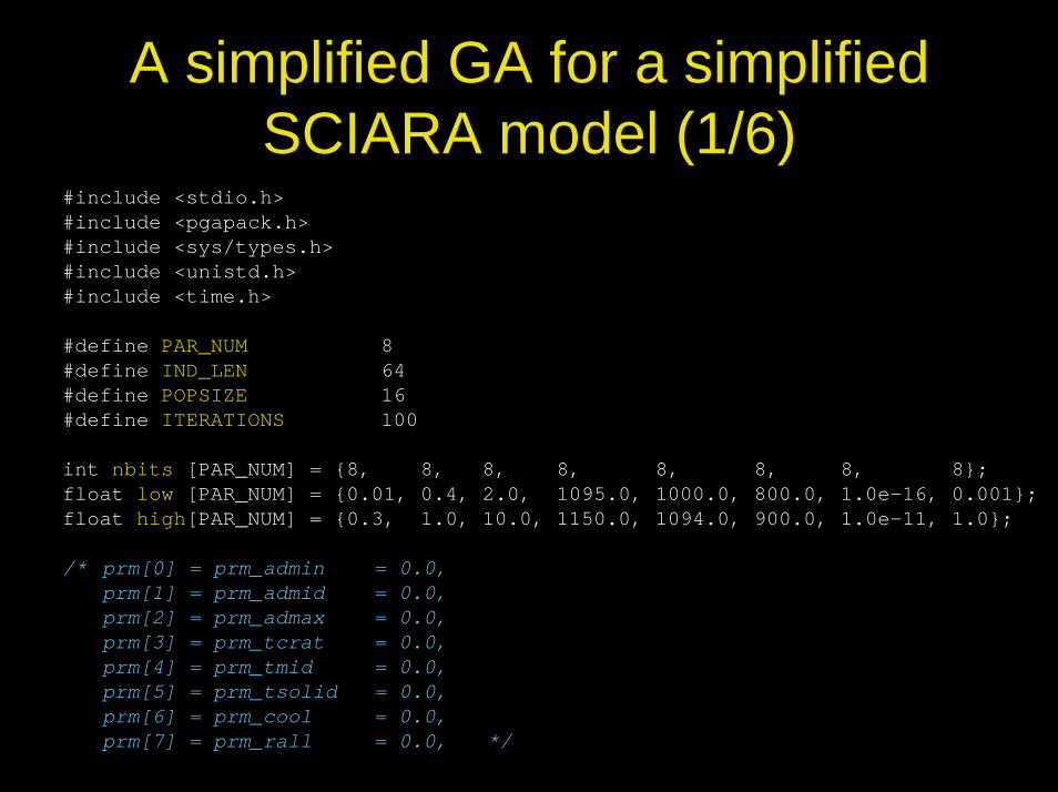
A simplified GA for a simplified SCIARA model (1/6)
#include <stdio.h>#include <pgapack.h>#include <sys/types.h>#include <unistd.h>#include <time.h>
#define PAR_NUM 8#define IND_LEN 64#define POPSIZE 16#define ITERATIONS 100
int nbits [PAR_NUM] = {8, 8, 8, 8, 8, 8, 8, 8};float low [PAR_NUM] = {0.01, 0.4, 2.0, 1095.0, 1000.0, 800.0, 1.0e-16, 0.001};float high[PAR_NUM] = {0.3, 1.0, 10.0, 1150.0, 1094.0, 900.0, 1.0e-11, 1.0};
/* prm[0] = prm_admin = 0.0,prm[1] = prm_admid = 0.0,prm[2] = prm_admax = 0.0,prm[3] = prm_tcrat = 0.0,prm[4] = prm_tmid = 0.0,prm[5] = prm_tsolid = 0.0,prm[6] = prm_cool = 0.0,prm[7] = prm_rall = 0.0, */
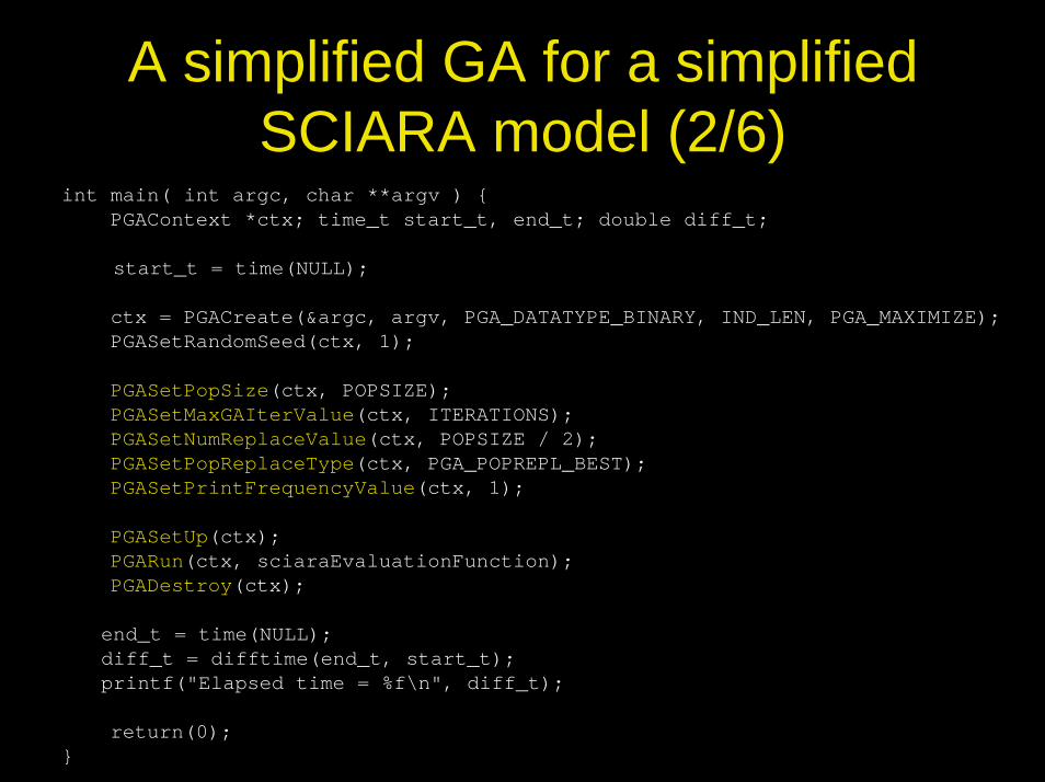
A simplified GA for a simplified SCIARA model (2/6)
int main( int argc, char **argv ) {PGAContext *ctx; time_t start_t, end_t; double diff_t;
start_t = time(NULL);
ctx = PGACreate(&argc, argv, PGA_DATATYPE_BINARY, IND_LEN, PGA_MAXIMIZE);PGASetRandomSeed(ctx, 1);
PGASetPopSize(ctx, POPSIZE);PGASetMaxGAIterValue(ctx, ITERATIONS);PGASetNumReplaceValue(ctx, POPSIZE / 2);PGASetPopReplaceType(ctx, PGA_POPREPL_BEST);PGASetPrintFrequencyValue(ctx, 1);
PGASetUp(ctx);PGARun(ctx, sciaraEvaluationFunction);PGADestroy(ctx);
end_t = time(NULL);diff_t = difftime(end_t, start_t);printf("Elapsed time = %f\n", diff_t);
return(0);}
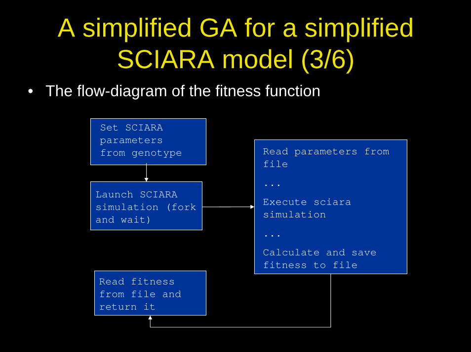
A simplified GA for a simplified SCIARA model (3/6)
• The flow-diagram of the fitness function
Set SCIARA parameters from genotype
Launch SCIARA simulation (fork and wait)
Read fitness from file and return it
Read parameters from file
...
Execute sciarasimulation
...
Calculate and save fitness to file
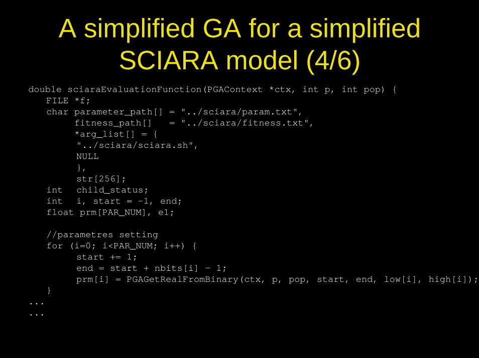
A simplified GA for a simplified SCIARA model (4/6)
double sciaraEvaluationFunction(PGAContext *ctx, int p, int pop) {FILE *f;char parameter_path[] = "../sciara/param.txt",
fitness_path[] = "../sciara/fitness.txt",*arg_list[] = {"../sciara/sciara.sh",NULL},str[256];
int child_status;int i, start = -1, end;float prm[PAR_NUM], e1;
//parametres settingfor (i=0; i<PAR_NUM; i++) {
start += 1;end = start + nbits[i] - 1;prm[i] = PGAGetRealFromBinary(ctx, p, pop, start, end, low[i], high[i]);
}......
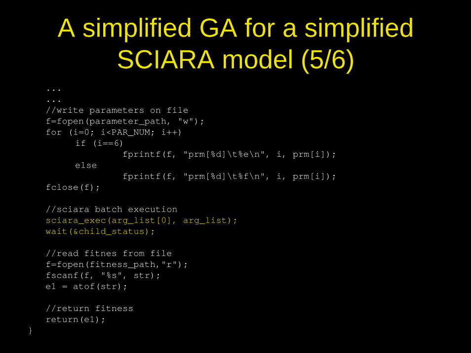
A simplified GA for a simplified SCIARA model (5/6)
...
...//write parameters on filef=fopen(parameter_path, "w");for (i=0; i<PAR_NUM; i++)
if (i==6)fprintf(f, "prm[%d]\t%e\n", i, prm[i]);
elsefprintf(f, "prm[%d]\t%f\n", i, prm[i]);
fclose(f);
//sciara batch executionsciara_exec(arg_list[0], arg_list);wait(&child_status);
//read fitnes from filef=fopen(fitness_path,"r");fscanf(f, "%s", str);e1 = atof(str);
//return fitnessreturn(e1);
}
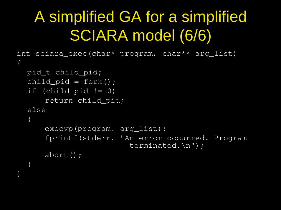
A simplified GA for a simplified SCIARA model (6/6)
int sciara_exec(char* program, char** arg_list){
pid_t child_pid;child_pid = fork();if (child_pid != 0)
return child_pid;else{
execvp(program, arg_list);fprintf(stderr, "An error occurred. Program
terminated.\n");abort();
}}
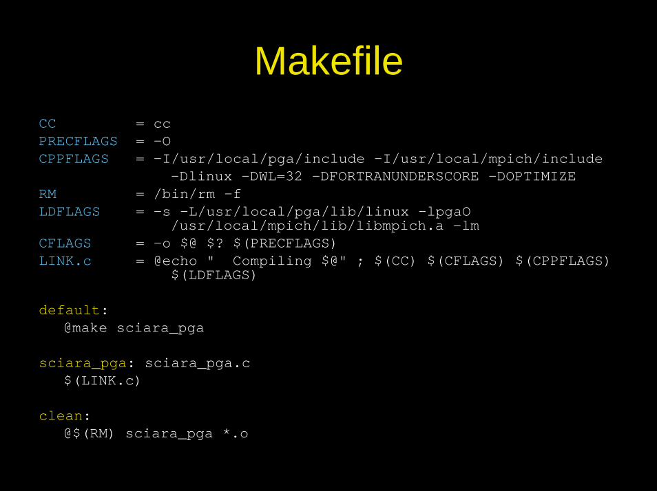
MakefileCC = ccPRECFLAGS = -O CPPFLAGS = -I/usr/local/pga/include -I/usr/local/mpich/include
-Dlinux -DWL=32 -DFORTRANUNDERSCORE -DOPTIMIZE RM = /bin/rm -fLDFLAGS = -s -L/usr/local/pga/lib/linux –lpgaO
/usr/local/mpich/lib/libmpich.a -lmCFLAGS = -o $@ $? $(PRECFLAGS)LINK.c = @echo " Compiling $@" ; $(CC) $(CFLAGS) $(CPPFLAGS)
$(LDFLAGS)
default:@make sciara_pga
sciara_pga: sciara_pga.c$(LINK.c)
clean: @$(RM) sciara_pga *.o
References• Crisci G. M., Di Gregorio S., Rongo R., Spataro, W., (2004). The simulation model
SCIARA: the 1991 and 2001 at Mount Etna. Journal of Vulcanogy and Geothermal Research, Vol 132/2-3, pp 253-267, 2004.
• D. D'Ambrosio, W. Spataro, and G. Iovine, in press. Parallel genetic algorithms foroptimising cellular automata models of natural complex phenomena: an application todebris-flows. Computer & Geosciences.
• D.E. Goldberg. Genetic Algorithms in Search, Optimization and Machine Learning. Addison-Wesley, 1989.
• J.H. Holland. Adaptation in Natural and Articial Systems. University of Michigan Press, Ann Arbor, 1975.
• G. Iovine, D. D'Ambrosio, and S. Di Gregorio, 2005. Applying genetic algorithms forcalibrating a hexagonal cellular automata model for the simulation of debris flowscharacterised by strong inertial effects. Geomorphology, 66, 287-303.
• J.R. Koza. Genetic Programming: On the Programming of Computers by Means of Natural Selection. MIT Press, 1992.
• M. Mitchell. An Introduction to Genetic Algorithms. MIT Press, 1996.• W. Spataro, D. D'Ambrosio, R Rongo and G.A. Trunfio, 2004. An Evolutionary
Approach for Modelling Lava Flows through Cellular Automata. In P.M.A. Sloot, B. Chopard and A.G.Hoekstra (Eds.), LNCS 3305, Proceedings ACRI 2004, University of Amsterdam, Science Park Amsterdam, The Netherlands, pp. 725-734.