Agro-ecoregionalization of Iowa using multivariate

geographical clustering

Carol L. Williams a,*, William W. Hargrove b, Matt Liebman a,David E. James c

a Department of Agronomy, Iowa State University, Ames, IA 50011, USAb USDA Forest Service, Southern Research Station, Building 1507, Room 211, Mail Stop 6407, Oak Ridge, TN 37831-6407, USA

c National Soil Tilth Lab, United States Department of Agriculture, Ames, IA 50011, USA

Received 27 December 2006; received in revised form 30 May 2007; accepted 1 June 2007

Available online 13 August 2007

Abstract

Agro-ecoregionalization is categorization of landscapes for use in crop suitability analysis, strategic agroeconomic development, risk

analysis, and other purposes. Past agro-ecoregionalizations have been subjective, expert opinion driven, crop specific, and unsuitable for

statistical extrapolation. Use of quantitative analytical methods provides an opportunity for delineation of agro-ecoregions in a more objective

and reproducible manner, and with use of generalized crop-related environmental inputs offers an opportunity for delineation of regions with

broader application. For this study, raster (cell-based) environmental data at 1 km scale were used in a multivariate geographic clustering

process to delineate agroecozones. Environmental parameters included climatic, edaphic and topographic characteristics hypothesized to be

generally relevant to many crops. Clustering was performed using five a priori grouping schemes of 5–25 agroecozones. Non-contiguous

geographic zones were defined representing areas of similar crop-relevant environmental conditions. A red–green–blue color triplet was used

for visualization of agroecozones as unique combinations of environmental factors. Concordance of the agroecozones with other widely used

datasets was investigated using MapCurves, a quantitative goodness-of-fit method. The 5- and 25-agroecozone schemes had highest

concordance with a map of major land resource areas and a map of major landform regions, with degree of fit judged to be good. The resulting

agroecozones provide a framework for future rigorous hypothesis testing. Other applications include: quantitative evaluation of crop

suitability at the landscape scale, environmental impact modeling and agricultural scenario building.

# 2007 Elsevier B.V. All rights reserved.

www.elsevier.com/locate/agee

Agriculture, Ecosystems and Environment 123 (2008) 161–174

Keywords: Agroecopause; Agroecozone; MapCurves; Multivariate geographic clustering

1. Introduction

Identification of relatively homogenous regions of

expected crop performance within landscapes has potential

benefits for improved agricultural policy formation and

resource conservation (USDA, 2006). Agro-ecoregionaliza-

tion has been used to identify land resource potentials and

limitations relevant to agriculture in spatially explicit terms.

Agroecozones (AEZs) serve as fundamental geographic

units providing information on the location and extent of

* Corresponding author. Tel.: +1 515 294 6735.

E-mail address: willico@iastate.edu (C.L. Williams).

0167-8809/$ – see front matter # 2007 Elsevier B.V. All rights reserved.

doi:10.1016/j.agee.2007.06.006

crop-relevant resources, their capabilities, and the potential

for future uses as part of strategic planning (Fan et al., 2000;

Swinton et al., 2001; Liu and Samal, 2002; Munier et al.,

2004; Patel, 2004). Previous AEZ delineations (e.g., FAO,

1996; Caldiz et al., 2001; Swinton et al., 2001) have been

crop specific, utilizing detailed information on crop

requirements, and have relied on expert opinion and

hierarchical frameworks. Regionalizations that depend on

observer interpretations on the basis of personal experience

are unsuitable for statistical extrapolation (Metzger et al.,

2005). Hierarchical approaches are affected by the order of

inputs, and require the subsuming of lower-level processes

within higher order regions, which requires a priori

C.L. Williams et al. / Agriculture, Ecosystems and Environment 123 (2008) 161–174162

understanding of landscape structure and function (Liu and

Samal, 2002; Zhou et al., 2003). Regions defined by these

methods then, are highly, if not entirely subjective, and are

generally not reproducible (Bunce et al., 1996; Bernert et al.,

1997; Swinton et al., 2001; Liu and Samal, 2002; Leathwick

et al., 2003; Hargrove and Hoffman, 2004; Thompson et al.,

2005). Additionally, traditional AEZ delineation approaches

fail to identify transition zones between AEZs (Liu and

Samal, 2002), adding further ambiguity to boundary

location and meaning. To use statistical inference in

landscape analysis of agricultural problems, stratification

of land into relatively homogenous regions using an

objective aggregation approach is necessary (Metzger

et al., 2005).

Crop growth simulation models have been used to predict

crop yields, and would seem to lend themselves to AEZ

delineation. While these process-based models provide

excellent yield forecasting within fields, they have limited

application across large geographic regions because: (1) the

point-like experimental plots upon which they are para-

meterized are not representative of environmental condi-

tions of larger areas (Kravchenko and Bullock, 2000; DeWit

et al., 2005); and, (2) many models are based on ideally

managed crop systems generally not representative of

environmental and management heterogeneity within

regions (Wassenaar et al., 1999; Hansen and Jones, 2000;

Batchelor et al., 2002; Viglizzo et al., 2004).

In response to the limitations of expert opinion-based

modeling, hierarchical frameworks, and location-specific

process-based growth models, a number of analytical

methods of regionalization have been developed with

applicability to agroecozoning. Multivariate models are

popular owing to the particular advantages of objectivity

and explicitness, greater defensibility, and improved

transferability (Hargrove and Hoffman, 2004; Pullar

et al., 2005). Growth in computing power and increased

availability of spatially explicit environmental data has

made the analytical approaches increasingly feasible

(Leathwick et al., 2003; Zhou et al., 2003). Geographic

information systems (GIS) have also been critical to the

development of regionalization models (Pariyar and Singh,

1994; Ghaffari et al., 2000; Patel, 2004). Geographic

information systems enable use of spatial data in a digital

environment, integration of data from separate scales, and

have application for data developed for agricultural

research (Corbett, 1996). While GIS reduces subjectivity

in the delineation process, its use is no guarantee of

objectivity if ‘‘manual methods’’ or other expert opinion-

driven methods are simply transferred to the digital

environment. Use of multivariate models in combination

with GIS, however, may offer improvements toward greater

objectivity and repeatability.

States within the U.S. Midwest are rapidly transforming

their economies to embrace bio-based industries such as

biofuel production (e.g., CIRAS, 2002; Battelle, 2004).

Crops not currently grown as commodities are likely to be

important elements of this transformation. Limiting factors

of potential alternative crops may not be well understood

across the entire range of adaptation, and therefore may be

problematic for traditional AEZ delineation methods (FAO,

1996). For example, switchgrass (Panicum virgatum), a

perennial grass currently under scrutiny as a potential

dedicated energy crop, is a highly variable species with a

wide range of ecotypes (Boe, 2003). Significant manage-

ment � cultivar � environment interactions that affect sur-

vival, growth and yield have been reported (Sanderson et al.,

1999; Lemus et al., 2002; Casler and Boe, 2003; Heaton

et al., 2004; Van Esbroeck et al., 2003; Berdahl et al., 2005;

Casler, 2005; Cassida et al., 2005; Lee and Boe, 2005;

Virgilio et al., 2007). Therefore, a method for producing

more generalized AEZs, as an alternative to traditionally

delineated AEZs, may be beneficial.

The purpose of this study was to delineate AEZs using a

quantitative analytical approach. The aim was to identify

different combinations of environmental factors as

distributed spatial units of similar potentials and limita-

tions, and that would have broad application to numerous

crops, including potential alternative crops. We defined

AEZs as areas of similarity of combined crop-relevant

climatic, topographic and edaphic conditions. Principal

components analysis (PCA), and multivariate geographic

clustering (MGC) in combination with a red–green–blue

color triplet were used to delineate AEZs (Hargrove and

Hoffman, 1999, 2004). Capture, storage, and preliminary

preparation of digital environmental data were conducted

in a GIS. Visualization and display of the AEZs were also

conducted in the GIS. A quantitative comparison with two

existing categorical land regionalizations was conducted

using a goodness-of-fit model. We use Iowa, USA, as a

case study to demonstrate our method and its potential

applications.

2. Materials and methods

2.1. Study area

The study area was Iowa, USA, a world leader in corn

(Zea mays L.) and soy (Glycine max) production (IDALS,

2004). Iowa is located between 89.58 and 96.58 west

longitude, and 40.58 and 43.58 north latitude. Total area of

Iowa is 145,743 km2, and elevation ranges from 146 to

509 m above mean sea level. Iowa’s climate is humid

continental, moist year round with long, hot summers

(Strahler and Strahler, 1984). Principal soil orders are

mollisols, alfisols, inceptisols and entisols (NRCS, 1999).

About 89% of the land area of Iowa is in cultivation, and

corn and soybean account for 93% of total land area

harvested (IDALS, 2004). Iowa is likely to experience major

agricultural transformation in the 21st century in response to

perceived bio-based economic opportunities (ISU Biore-

newables Office, 2003).

C.L. Williams et al. / Agriculture, Ecosystems and Environment 123 (2008) 161–174 163

2.2. Development of the environmental dataset

We have taken a ‘‘generic’’ approach in quantitative

regionalization of land resources by including in our models

environmental parameters hypothesized to be potentially

growth limiting for a wide variety of crops. Our aim was to

categorize land resources in a way that is relevant to crops

which are functionally, anatomically, and physiologically

different from each other (i.e., have different limiting

factors). Parameters chosen for the dataset were based on

those described by Nix (1981), Loomis and Connor (1992),

Prentice et al. (1992), Booth (1996), FAO (1996), and Young

et al. (1999). Mean values of environmental predictors

within spatial units of analysis (e.g., raster cells) were

reasoned to be relevant to crop performance within spatial

units. Variability, or dependability, of environmental

parameters within analysis units was also reasoned to be

relevant to crops. Therefore, standard deviations of

environmental parameters were included in the dataset.

Environmental parameters fell into three categories:

climatic, topographic, and edaphic. Environmental data

were obtained digitally and subsequently stored, managed,

manipulated, and displayed in ArcGIS 9.1 (ESRI, 2005).

Eight climate parameters were included in the models

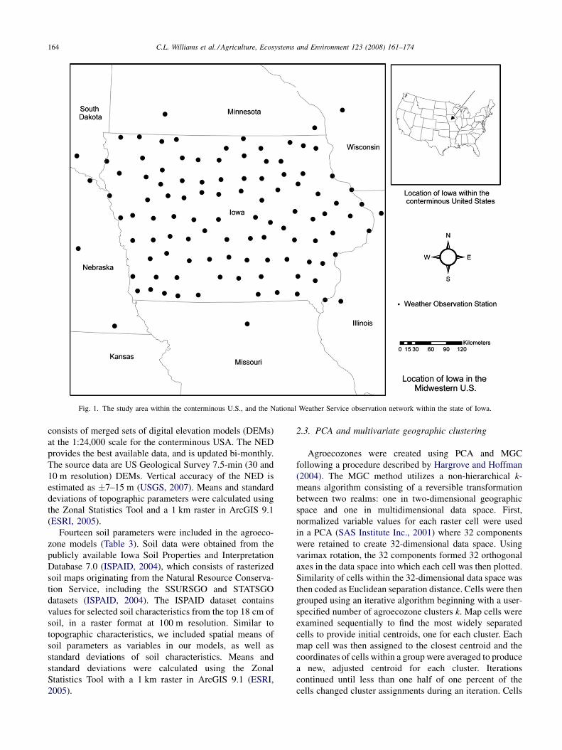
(Table 1). Climate parameters were derived from daily

weather observations for the period 1985–2004, at 98

National Weather Service Cooperative Stations (NWSCS)

evenly distributed across Iowa (Fig. 1; IEM, 2005). This

network provides the highest spatial density of observations

for the parameters of interest and for the period of

observation. To widen the inference window beyond state

boundaries, daily weather data from ten additional NWSCS

among the six adjacent states were included in the dataset

(Fig. 1; HPRCC, 2005; MRCC, 2005; MCC, 2005).

Growing season was determined for each observation

station as the number of days between the mean day-of-

year in spring with less than 20% chance of the air

temperature falling below 0 8C, and mean day-of-year in fall

with a greater than 20% chance of the air temperature

dropping below 0 8C. Climate parameters were calculated as

Table 1

Summary of climate parameters

Parameter Units

Mean annual precipitation mm

Standard deviation of mean annual precipitation

Mean growing season length Days

Standard deviation of mean growing season length

Mean growing season precipitation mm

Standard deviation of mean growing season precipitation

Mean growing season heat units 8C

Standard deviation of mean growing season heat units

means and standard deviations across the period of

observation. Mean and standard deviation values of climate

parameters at each observation station were then used to

interpolate a raster surface of 1 km resolution using ordinary

kriging (ArcGIS 9.1 Geostatistical Analyst; ESRI, 2005).

Kriging has been shown to have better results than other

methods of spatial interpolation for estimating climate

characteristics, and to be visually more plausible (Collins

and Bolstad, 1999). The kriging method of spatial

interpolation was therefore chosen for its conceptual

straightforwardness, suitability for the data, and interactive

modeling approach in ArcGIS (9.1; ESRI, 2005). For each

climate parameter an iterative process was used to create the

best-fit model (e.g., least weighted squared error). Inter-

polation included a maximum of six neighbors (minimum of

three). In each case the spherical model provided the best fit,

and residuals were randomly distributed. An example of the

spatial distribution of prediction error is presented in Fig. 2.

Ten topographic parameters were included in the models

(Table 2). Many topographic characteristics can be

described as ‘‘spatially permanent’’. That is, such char-

acteristics change very little over time, especially compared

to weather and climate, which change more rapidly over

time at a location. The mean of a topographic characteristic

within a spatial unit is useful for making comparisons among

spatial units. However, we argue that amount of dispersion

around a mean is also a desirable description of hetero-

geneity of spatially permanent environmental characteris-

tics. For example, two spatial units may have the same mean

elevation, but very different standard deviations. A spatial

unit with higher standard deviation of mean elevation has

greater topographic relief than a spatial unit with smaller

standard deviation. This type of difference among spatial

units may be relevant to differences in crop productivity

among spatial units. Therefore, means and standard

deviations of topographic characteristics are included in

the models. Topographic parameters were derived from the

publicly available national elevation dataset (NED; USGS,

1999) in raster format at 30 m resolution, and resampled to

100 m resolution (ArcGIS 9.1; ESRI, 2005). The NED

Description

Total annual precipitation averaged for 1985–2004

Amount of interannual variability of total precipitation

Total number of days between date in spring of 20%

or less probability of frost, and date in fall with 20%

or greater probability of frost, averaged for 1985–2004

Amount of interannual variability of growing season length

Total precipitation between frost-free dates, averaged for

1985–2004

Amount of interannual variability of growing season precipitation

Total number of 8C above 08, between frost-free dates, averaged

for 1985–2004

Amount of interannual variability of growing season heat units

C.L. Williams et al. / Agriculture, Ecosystems and Environment 123 (2008) 161–174164

Fig. 1. The study area within the conterminous U.S., and the National Weather Service observation network within the state of Iowa.

consists of merged sets of digital elevation models (DEMs)

at the 1:24,000 scale for the conterminous USA. The NED

provides the best available data, and is updated bi-monthly.

The source data are US Geological Survey 7.5-min (30 and

10 m resolution) DEMs. Vertical accuracy of the NED is

estimated as �7–15 m (USGS, 2007). Means and standard

deviations of topographic parameters were calculated using

the Zonal Statistics Tool and a 1 km raster in ArcGIS 9.1

(ESRI, 2005).

Fourteen soil parameters were included in the agroeco-

zone models (Table 3). Soil data were obtained from the

publicly available Iowa Soil Properties and Interpretation

Database 7.0 (ISPAID, 2004), which consists of rasterized

soil maps originating from the Natural Resource Conserva-

tion Service, including the SSURSGO and STATSGO

datasets (ISPAID, 2004). The ISPAID dataset contains

values for selected soil characteristics from the top 18 cm of

soil, in a raster format at 100 m resolution. Similar to

topographic characteristics, we included spatial means of

soil parameters as variables in our models, as well as

standard deviations of soil characteristics. Means and

standard deviations were calculated using the Zonal

Statistics Tool with a 1 km raster in ArcGIS 9.1 (ESRI,

2005).

2.3. PCA and multivariate geographic clustering

Agroecozones were created using PCA and MGC

following a procedure described by Hargrove and Hoffman

(2004). The MGC method utilizes a non-hierarchical k-

means algorithm consisting of a reversible transformation

between two realms: one in two-dimensional geographic

space and one in multidimensional data space. First,

normalized variable values for each raster cell were used

in a PCA (SAS Institute Inc., 2001) where 32 components

were retained to create 32-dimensional data space. Using

varimax rotation, the 32 components formed 32 orthogonal

axes in the data space into which each cell was then plotted.

Similarity of cells within the 32-dimensional data space was

then coded as Euclidean separation distance. Cells were then

grouped using an iterative algorithm beginning with a user-

specified number of agroecozone clusters k. Map cells were

examined sequentially to find the most widely separated

cells to provide initial centroids, one for each cluster. Each

map cell was then assigned to the closest centroid and the

coordinates of cells within a group were averaged to produce

a new, adjusted centroid for each cluster. Iterations

continued until less than one half of one percent of the

cells changed cluster assignments during an iteration. Cells

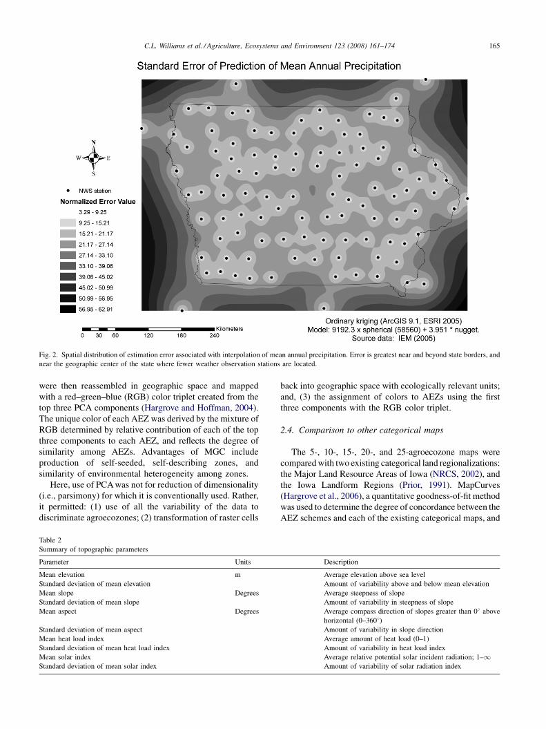
C.L. Williams et al. / Agriculture, Ecosystems and Environment 123 (2008) 161–174 165

Fig. 2. Spatial distribution of estimation error associated with interpolation of mean annual precipitation. Error is greatest near and beyond state borders, and

near the geographic center of the state where fewer weather observation stations are located.

were then reassembled in geographic space and mapped

with a red–green–blue (RGB) color triplet created from the

top three PCA components (Hargrove and Hoffman, 2004).

The unique color of each AEZ was derived by the mixture of

RGB determined by relative contribution of each of the top

three components to each AEZ, and reflects the degree of

similarity among AEZs. Advantages of MGC include

production of self-seeded, self-describing zones, and

similarity of environmental heterogeneity among zones.

Here, use of PCA was not for reduction of dimensionality

(i.e., parsimony) for which it is conventionally used. Rather,

it permitted: (1) use of all the variability of the data to

discriminate agroecozones; (2) transformation of raster cells

Table 2

Summary of topographic parameters

Parameter Units

Mean elevation m

Standard deviation of mean elevation

Mean slope Degrees

Standard deviation of mean slope

Mean aspect Degrees

Standard deviation of mean aspect

Mean heat load index

Standard deviation of mean heat load index

Mean solar index

Standard deviation of mean solar index

back into geographic space with ecologically relevant units;

and, (3) the assignment of colors to AEZs using the first

three components with the RGB color triplet.

2.4. Comparison to other categorical maps

The 5-, 10-, 15-, 20-, and 25-agroecozone maps were

compared with two existing categorical land regionalizations:

the Major Land Resource Areas of Iowa (NRCS, 2002), and

the Iowa Landform Regions (Prior, 1991). MapCurves

(Hargrove et al., 2006), a quantitative goodness-of-fit method

was used to determine the degree of concordance between the

AEZ schemes and each of the existing categorical maps, and

Description

Average elevation above sea level

Amount of variability above and below mean elevation

Average steepness of slope

Amount of variability in steepness of slope

Average compass direction of slopes greater than 08 above

horizontal (0–3608)Amount of variability in slope direction

Average amount of heat load (0–1)

Amount of variability in heat load index

Average relative potential solar incident radiation; 1–1Amount of variability of solar radiation index

C.L. Williams et al. / Agriculture, Ecosystems and Environment 123 (2008) 161–174166

Table 3

Summary of soil parameters

Parameter Units Description

Mean plant-available water capacity mm Average water capacity

Standard deviation of mean plant-available

water capacity

Amount of variability of mean plant available water

capacity

Mean cation exchange capacity mequiv./100 g soil Average cation exchange capacity

Standard deviation of mean cation exchange

capacity

Amount of variability of cation exchange capacity

Mean organic matter % Average percent of organic matter within the surface

horizon

Standard deviation of mean organic matter Amount of variability of mean organic matter

Mean permeability mm/h Average rate of water infiltration

Standard deviation of mean permeability Amount of variability of permeability

Mean of low value of pH range Average low value of the pH range

Standard deviation of mean low value of pH range Amount of variability of mean low value of pH range

Mean percent sand % Average percent sand

Standard deviation of mean percent sand Amount of variability of percent sand

Mean depth to seasonally high water table m Average depth to seasonally high water table

Standard deviation of mean depth to seasonally

high water table

Amount of variability of depth to seasonally high water

table

for comparing the two existing categorical maps with each

other. MapCurves (Hargrove et al., 2006) is resolution

dependent and is based on categories (rather than cell-by-cell

comparison), and therefore does not require that maps being

compared have identical number or types of categories. The

method determines the degree of spatial overlap, or positive

spatial correlation, between two or more maps with the same

spatial extent by using a goodness-of-fit algorithm according

to the equation:

g ¼X��

C

Bþ C

��C

Aþ C

��

where g is the goodness-of-fit score, C the amount of

intersection of a category between two maps; B the total

area of the category on a reference map; and A is the total

area of the category on the compared map. The first term

provides the proportion of category sharedness between

maps, and the second term weights by fractional share of

category area. (Weighting prevents distortion of fit by pre-

sence of many large, but minimally intersecting categories.)

The goodness-of-fit score is the sum of positive spatial

correlation among categories between two maps, and ranges

between 0 and 100, with higher scores indicating better fit.

3. Results and discussion

The number of AEZs chosen for this study were 5, 10, 15,

20, and 25, providing five portrayals of a landscape at

increasing level of detail. In moving from one portrayal to

another, all cells were reassigned to a new scheme of

clusters. Therefore, the AEZs are non-hierarchical. The non-

hierarchical method of MGC does not rely on preconceived

notions of landscape structure and allows a uniform

classification structure to emerge from the data by using

the variance structure present in environmental parameters

(Hargrove and Hoffman, 2004).

Raster cells were given a cluster assignment based on

location in data space regardless of absolute geographic

location. This resulted in fragmented AEZs composed of

spatially disjoined patches of varying size and of varying

distances between patches. Cohesiveness results from

spatial autocorrelation present in the environmental data

while fragmentation results from cells of differing geo-

graphic location having nearby locations in data space.

Simultaneous cohesiveness and fragmentation are desirable

for three reasons: (1) these properties reveal the non-random

organization of the agro-environment; (2) distributed areas

of crop-relevant environmental similarity are identifiable

with the methodology; and, (3) transitions between AEZs

are complex, which may be more representative of existing

environmental heterogeneity than discrete boundary lines

(McDonald et al., 2005). These desirable outcomes are

addressed in further detail below in a discussion of the 5-,

15-, and 25-zone schemes. For brevity, the 10- and 20-zone

schemes are not discussed here, but are presented together

with the 5-, 15- and 25-zone schemes on-line at http://

research.esd.ornl.gov/�hnw/iowa.

3.1. PCA axes and RGB color triplets

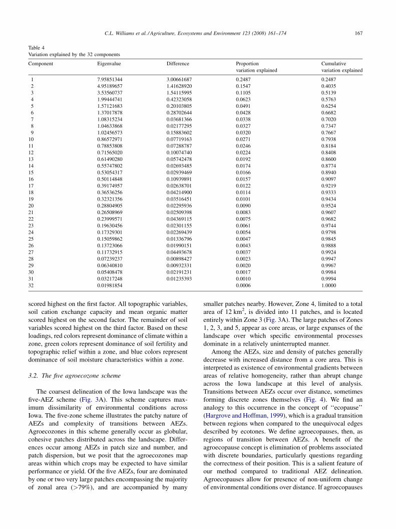
All 32 components were retained from the PCA and

formed the axes of the data space. The relative contribution

of each component is provided in Table 4, with the all of the

variation being captured by the 32 components (i.e.,

cumulative variation explained = 1.00). Varimax rotation

(orthogonal) factor loadings were used to interpret the first,

second and third principal components, which were used to

create the RGB color triplets (Table 5). Climate variables

C.L. Williams et al. / Agriculture, Ecosystems and Environment 123 (2008) 161–174 167

Table 4

Variation explained by the 32 components

Component Eigenvalue Difference Proportion

variation explained

Cumulative

variation explained

1 7.95851344 3.00661687 0.2487 0.2487

2 4.95189657 1.41628920 0.1547 0.4035

3 3.53560737 1.54115995 0.1105 0.5139

4 1.99444741 0.42323058 0.0623 0.5763

5 1.57121683 0.20103805 0.0491 0.6254

6 1.37017878 0.28702644 0.0428 0.6682

7 1.08315234 0.03681366 0.0338 0.7020

8 1.04633868 0.02177295 0.0327 0.7347

9 1.02456573 0.15883602 0.0320 0.7667

10 0.86572971 0.07719163 0.0271 0.7938

11 0.78853808 0.07288787 0.0246 0.8184

12 0.71565020 0.10074740 0.0224 0.8408

13 0.61490280 0.05742478 0.0192 0.8600

14 0.55747802 0.02693485 0.0174 0.8774

15 0.53054317 0.02939469 0.0166 0.8940

16 0.50114848 0.10939891 0.0157 0.9097

17 0.39174957 0.02638701 0.0122 0.9219

18 0.36536256 0.04214900 0.0114 0.9333

19 0.32321356 0.03516451 0.0101 0.9434

20 0.28804905 0.02295936 0.0090 0.9524

21 0.26508969 0.02509398 0.0083 0.9607

22 0.23999571 0.04369115 0.0075 0.9682

23 0.19630456 0.02301155 0.0061 0.9744

24 0.17329301 0.02269439 0.0054 0.9798

25 0.15059862 0.01336796 0.0047 0.9845

26 0.13723066 0.01990151 0.0043 0.9888

27 0.11732915 0.04493678 0.0037 0.9924

28 0.07239237 0.00898427 0.0023 0.9947

29 0.06340810 0.00932331 0.0020 0.9967

30 0.05408478 0.02191231 0.0017 0.9984

31 0.03217248 0.01235393 0.0010 0.9994

32 0.01981854 0.0006 1.0000

scored highest on the first factor. All topographic variables,

soil cation exchange capacity and mean organic matter

scored highest on the second factor. The remainder of soil

variables scored highest on the third factor. Based on these

loadings, red colors represent dominance of climate within a

zone, green colors represent dominance of soil fertility and

topographic relief within a zone, and blue colors represent

dominance of soil moisture characteristics within a zone.

3.2. The five agroecozone scheme

The coarsest delineation of the Iowa landscape was the

five-AEZ scheme (Fig. 3A). This scheme captures max-

imum dissimilarity of environmental conditions across

Iowa. The five-zone scheme illustrates the patchy nature of

AEZs and complexity of transitions between AEZs.

Agroecozones in this scheme generally occur as globular,

cohesive patches distributed across the landscape. Differ-

ences occur among AEZs in patch size and number, and

patch dispersion, but we posit that the agroecozones map

areas within which crops may be expected to have similar

performance or yield. Of the five AEZs, four are dominated

by one or two very large patches encompassing the majority

of zonal area (>79%), and are accompanied by many

smaller patches nearby. However, Zone 4, limited to a total

area of 12 km2, is divided into 11 patches, and is located

entirely within Zone 3 (Fig. 3A). The large patches of Zones

1, 2, 3, and 5, appear as core areas, or large expanses of the

landscape over which specific environmental processes

dominate in a relatively uninterrupted manner.

Among the AEZs, size and density of patches generally

decrease with increased distance from a core area. This is

interpreted as existence of environmental gradients between

areas of relative homogeneity, rather than abrupt change

across the Iowa landscape at this level of analysis.

Transitions between AEZs occur over distance, sometimes

forming discrete zones themselves (Fig. 4). We find an

analogy to this occurrence in the concept of ‘‘ecopause’’

(Hargrove and Hoffman, 1999), which is a gradual transition

between regions when compared to the unequivocal edges

described by ecotones. We define agroecopauses, then, as

regions of transition between AEZs. A benefit of the

agroecopause concept is elimination of problems associated

with discrete boundaries, particularly questions regarding

the correctness of their position. This is a salient feature of

our method compared to traditional AEZ delineation.

Agroecopauses allow for presence of non-uniform change

of environmental conditions over distance. If agroecopauses

C.L. Williams et al. / Agriculture, Ecosystems and Environment 123 (2008) 161–174168

Table 5

Varimax rotation scores on the first three components of PCA

Parameter Factor 1

(red)

Factor 2

(green)

Factor 3

(blue)

Mean annual precipitation 0.869 0.025 0.166

Standard deviation of mean annual precipitation 0.854 �0.096 0.013

Mean growing season length 0.887 0.128 �0.090

Standard deviation of growing season length 0.841 0.211 �0.096

Mean growing season precipitation 0.780 �0.068 0.071

Standard deviation of growing season precipitation 0.920 0.057 0.020

Mean growing season heat units 0.822 0.058 �0.107

Standard deviation of growing season heat units 0.758 0.178 0.035

Mean plant available water capacity �0.071 �0.008 �0.640

Standard deviation of available water capacity 0.04 0.178 0.727

Mean cation exchange capacity �0.209 �0.500 �0.389

Standard deviation of cation exchange capacity �0.124 �0.512 0.573

Mean organic matter �0.179 �0.513 0.001

Standard deviation of organic matter �0.176 �0.316 0.365

Mean permeability �0.037 0.085 0.455

Standard deviation of permeability 0.052 0.213 0.622

Mean low value of pH range �0.409 �0.307 0.094

Standard deviation of low value of pH range �0.302 �0.153 0.353

Mean percent sand �0.053 �0.137 0.699

Standard deviation of percent sand 0.285 0.070 0.677

Mean depth to seasonal water table �0.129 0.503 �0.031

Standard deviation of depth to water table 0.085 �0.314 0.478

Mean elevation �0.779 �0.077 �0.220

Standard deviation of elevation 0.060 0.886 0.014

Mean slope 0.072 0.802 0.001

Standard deviation of slope 0.148 0.862 0.093

Mean aspect 0.026 0.028 �0.043

Standard deviation of aspect 0.003 0.028 0.051

Mean heat load index 0.004 �0.551 �0.048

Standard deviation of heat load index 0.159 0.896 �0.046

Mean solar radiation index 0.005 �0.555 �0.047

Standard deviation of solar radiation index 0.179 0.892 �0.015

are significant elements of the landscape, they present

additional features to be considered in agricultural planning

and policy. For example, current field-level cultural

practices are unlikely to increase biodiversity (Moser

et al., 2002). However, crop diversification for increased

biodiversity could be planned at the landscape level.

Agoecopauses may represent spatial units of greater

potential crop diversity and could be targeted for enhancing

agro-biodiversity goals.

3.3. The 15 agroecozone scheme

In the 15-zone scheme (Fig. 3B), AEZs are again patchy,

but are of globular and linear shapes. In this scheme, five

AEZs dominate in terms of total area (Zones 1, 8, 10, 12, and

13), each composed of one or two large patches encom-

passing >77% of each zonal area. The remaining AEZs

occupy substantially less area distributed among many small

patches. This zonation illustrates how the study landscape is

composed of diverse subregions of dominant environmental

components and processes.

Zones 1 and 15 present an interesting opportunity for

interpretation of crop-relevant environmental variation at the

subregional scale. Zone 1, composed of 386 patches, lacks a

single core area. It contains two large globular patches

comprising 92.9% of the zonal area separated by a distance

of approximately 118 km and five intervening AEZs.

Despite the amount of distance between these two patches,

they are more similar to each other than any of the other

AEZs. A similar amount of patch dispersal is present in Zone

15 which is composed on many linear patches. Zone 15 also

lacks a core area in terms of a discrete compact patch near

the geographic center of the zone. Zone 5 contains hundreds

widely disperesed small patches juxtaposed with larger very

dissimilar AEZs (Fig. 5). The larger surrounding AEZs,

then, are an intervening matrix of complex environmental

conditions. This combination of widely dispersed patches

amidst a complex matrix of environmental heterogeneity

may provide a tool for understanding biodiversity and

conservation opportunities at the landscape scale. Small

distributed patches may offer locations for introduction of

specialty crops, for example, into wider more homogenous

regions of conventional commodity crops.

3.4. The 25-agroecozone scheme

The 25-zone scheme (Fig. 3C) presents a very detailed

picture of the crop-relevant environment within the study

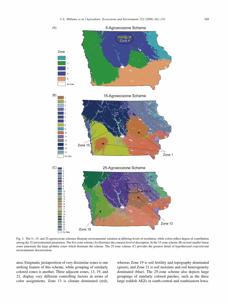
C.L. Williams et al. / Agriculture, Ecosystems and Environment 123 (2008) 161–174 169

Fig. 3. The 5-, 15- and 25-agroecozone schemes illustrate environmental variation at differing levels of resolution, while colors reflect degree of contribution

among the 32 environmental parameters. The five-zone scheme (A) illustrates the coarsest level of description. In the 15-zone scheme (B) several smaller linear

zones punctuate the large globular zones which dominate the scheme. The 25-zone scheme (C) provides the greatest detail of hypothesized crop-relevant

environmental discretization.

area. Enigmatic juxtaposition of very dissimilar zones is one

striking feature of this scheme, while grouping of similarly

colored zones is another. Three adjacent zones, 13, 19, and

21, display very different controlling factors in terms of

color assignments. Zone 13 is climate dominated (red),

whereas Zone 19 is soil fertility and topography dominated

(green), and Zone 21 is soil moisture and soil heterogeneity

dominated (blue). The 25-zone scheme also depicts large

groupings of similarly colored patches, such as the three

large reddish AEZs in south-central and southeastern Iowa.

C.L. Williams et al. / Agriculture, Ecosystems and Environment 123 (2008) 161–174170

Fig. 4. Agroecopauses: boundaries are complex and transitions between agroecozones occur over considerable distances.

Although MGC results in non-hierarchical zones, these

groupings demonstrate how MGC organizes spatial units

simultaneously into generalizable environmental processes

and differentiated subregional expressions via color triplets.

This characteristic of the method could be beneficial to

policy makers and researchers alike, who may be interested

in simultaneous generalized and more detailed analyses.

Fig. 5. Distributed agroecozones. Zone 5 of the 15-zone scheme (shown in

black), typifies agroecozones which have small total area but are widely

distributed across the state. These agroecozones are surrounded by a matrix

of complex and often very dissimilar conditions.

3.5. Validity of the AEZs

An inherently desirable component of regionalization is

demonstrable validity (Lugo et al., 1999; Liu and Samal,

2002). However, generally accepted quantitative methods

for assessing correctness of eco-regionalization schemes, or

for estimating statistical significance of differences among

regions, do not exist (Hargrove and Hoffman, 2004).

Ground-truthing is a method that has been used to evaluate

whether ecological map units capture intended ecological

variables (Kupfer and Franklin, 2000). Unfortunately,

currently available yield data for crops grown throughout

the study area (e.g., corn and soy) are aggregated mean

yields at the county level (NASS, 2005). This resolution is

too coarse for AEZ validation, and counties and AEZs are

not of the same size or configuration, precluding one-to-one

comparisons.

Metzger et al. (2005) used comparison of their climatic

stratification of Europe with previously created classifica-

tions to evaluate credibility of their results. This is a tractable

approach if the reference maps are themselves validated. In

the case of Iowa land classification, two existing regiona-

lization maps are the Major Land Resource Areas of Iowa

(MLRAs; NRCS, 2002), and the Landform Regions of Iowa

(LRI; Prior, 1991). These maps are traditionally delineated

(e.g., subjectively derived) regionalizations of Iowa, and

their degree of validity has not been reported. Nonetheless,

C.L. Williams et al. / Agriculture, Ecosystems and Environment 123 (2008) 161–174 171

Table 6

Goodness-of-fit scores using MapCurves (Hargrove et al., 2006)

5-AEZ 10-AEZ 15-AEZ 20-AEZ 25-AEZ MLRAs LANDFORMS

5-AEZ 51.8 47.1 58.2 60.7 58.4 48.8

10-AEZ 39.5 40.0 38.7 27.6 29.4

15-AEZ 66.1 67.2 28.6 32.0

20-AEZ 58.5 37.1 39.6

25-AEZ 45.5 45.0

MLRAs 76.3

they are widely used in education and research as currently

best available sources of information (e.g., Bernert et al.,

1997; Waltman et al., 2004; Vogel et al., 2005). Using

MapCurves goodness-of-fit test (Hargrove et al., 2006), we

quantitatively evaluated concordance of the 5-, 10-, 15-, 20-,

and 25-AEZ schemes with each other, and with the MLRA

and LRI maps. We also measured concordance between the

MLRA and the LRI maps. Results are presented in Table 6.

When compared to the MLRAs and the LRI, the

descending rank order of the AEZ schemes is the same:

5, 25, 20, 15, and 10. The same order of fit among AEZ

schemes with the MLRAs and LRI is not surprising as the

degree of fit between the MLRAs and the LRI is 76.28, a

very high score. We expect this high degree of concordance

between MLRAs and LRI because the schemes use similar

criteria for determining regions and their boundaries (e.g.,

topography; USDA, 2006; Prior, 1991), and therefore are not

independent. The 5- and 25-AEZ schemes have better fit

with the MLRAs while the 10-, 15- and 20-AEZ schemes

have better fit with the ILR. The degree of fit of the 5- and

25-AEZ, the top ranking schemes, with both the MLRAs and

the ILR is ‘‘good’’. The 5- and 25-AEZ schemes have high

degree of concordance with each other (60.7), and therefore

their similar scores with the MLRAs and the LRI is not

surprising. The 10-AEZ scheme has the lowest concordance

with the MLRA (27.6), and the 15-AEZ scheme had the least

concordance with the LRI (28.6). Among AEZ schemes, the

highest degree of concordance is between the 20- and 25-

AEZ schemes (67.2), lowest is between the 10- and 25-AEZ

schemes (38.7).

The above measures of goodness-of-fit are not a measure

of correctness of any of the maps because: (1) it is difficult to

justify comparison of maps created for different purposes

and using differing criteria and methods (McMahon et al.,

2001; Thompson et al., 2005); and (2) as stated above, the

reference maps themselves have not been ‘‘validated’’.

Therefore, we interpret the results as a sign of an emerging

consensus.

Our method is straightforward, empirical and wholly

transferable. Expert opinion is required for choice of input

parameters, but this is a common feature of all analytical

models. Once inputs are chosen, however, our AEZ

delineation method is objective, ‘‘data driven’’. Data

dependency is in this case a positive outcome, indicating

the repeatability of the results. Validity of the AEZs can be

seen, then, as a function of the validity and quality of the

input data, and the choice of inputs. The data used in the

present study are digital and publicly available, and thus not

subject to the problems of distribution and physical

distortion associated with analogue data (e.g., paper maps)

used in previous AEZ methods. By using best currently

available data, our AEZ provide updated information

compared to previous regionalization schemes. Addition-

ally, our method would facilitate rapid updating of AEZs as

input data are revised over time.

There are limitations of this study that should be

considered, two of which are discussed here. It is very rare

that all data required for a given analysis are measured at the

same scale or over the same extent. Interpolation,

extrapolation, and aggregation of spatial data, all very

common procedures of geographic analysis, introduce

modeling error (Openshaw, 1977; MacEachren and David-

son, 1987). Currently, methods are unavailable for evaluat-

ing total error in a surface produced from multiple layers of

data as well as the propagation of error through each step in

surface building. As a result, the amount of total error in the

AEZs is unknown. Secondly, the degree to which existing or

future crops will respond to environmental variability

identified by the AEZs is unknown. Therefore, significance

of the environmental variability captured by our AEZs is

unknown. The degree of crop response and tolerance to

differences among AEZs must be determined in order to

assess the significance of differences among AEZs. Yields of

existing crops sampled for capture of regional differences, if

present, would be the best method to make this determina-

tion. Such efforts could be assisted by analysis of satellite

imagery, or other remotely sensed data.

3.6. Core applications

A major result of this study is quantification of the

environment relevant to crops using a wholly transferable

and empirical method. Use of a quantitative method to

categorize the environment makes possible the testing of

hypotheses of crop performance using environmental

parameters as non-random variables (i.e., using robust

statistical analysis). Agroecozones delineated by our method

make it possible, for example, to create an experimental

design for field tests of crops across a known range of

environmental conditions and combined environmental

factors. This makes possible the choice of trial locations

in a spatially explicit and analytical manner. Such a targeted

C.L. Williams et al. / Agriculture, Ecosystems and Environment 123 (2008) 161–174172

approach has the additional advantage of one-to-one

comparisons between measures of crop performance and

environmental characteristics across space. An essential

requirement for testing such hypotheses is experimental

design (i.e., distribution of samples) that measures regional-

scale ecological processes, not plot- or farm-level ecological

processes. Sample locations, for example, could be stratified

among AEZs, and randomized within AEZs. This approach

provides an alternative to the traditional agronomic

approach of field trials under idealized environmental and

management conditions that do not extrapolate well to

regional scales (Hansen and Jones, 2000; Batchelor et al.,

2002).

Agricultural land use decision-making is scale dependent

and must correspond to an appropriate level of agro-

ecosystem behavior (Veldkamp et al., 2001). A principal

core application of our AEZ delineation method is inventory

of crop-relevant environmental characteristics commensu-

rate with the needs of decision-making at higher levels of

socio-economic and political organization. At such levels

focus is on, for example, commodity quality demands,

sustainable land use planning, new crop introduction, and

regional economic development (Fan et al., 2000; Hansen

and Jones, 2000; Munier et al., 2004; Jagtap and Jones,

2002; Verdoodt and Van Ranst, 2006). Therefore, a primary

application of our method is evaluation of crop suitability.

Here, AEZs are delineated as relatively homogenous regions

of quantified environmental conditions. Specifically, the

landscape has been discretized on the basis of crop-relevant

environmental characteristics. If crop growth requirements

are even minimally understood, the AEZs provide a

screening tool in suitability analysis. Because the MGC

method results in AEZs with similar variance, they are better

suited for such an analysis than traditionally delineated AEZ

which have unknown and presumably unequal variances

among regions. In crop suitability analysis, future climate

conditions might be an important consideration. With the

MGC method, estimates of future climate characteristics can

be used as inputs in the same way that historical climate data

have been used in the present study. For more detailed

suitability analysis Patel (2004) recommends addition of

supplemental data layers to GIS-based AEZs. Data layers

containing particular limiting parameters could identify

areas within and among AEZs that exceed crop limits.

Unsuitable areas could then be masked from further

evaluation.

The MGC method of AEZ delineation using crop-

relevant environmental parameters could be a valuable

framework for agricultural scenario building (Santelmann

et al., 2006). Instead of bounding agroecological problems

by arbitrary administrative units (e.g., counties) or hydro-

logically defined areas (e.g., watersheds), AEZ boundaries

reflect ecological processes specific to agriculture. Together

with additional information such as infrastructure, popula-

tion structure, land ownership patterns, and water resources,

planners and policy makers could use AEZs to analyze

trade-offs associated with changes in policies affecting

agricultural production and resource conservation. AEZs

could similarly be used as agriculture-centric geographic

units for water quality management. If empirical models of

the effects of crops and associated management practices on

water quality are available, AEZs could be used to predict

how changes in crops and management may affect water

quality.

Agroecozones represent additional opportunities for

study of socio-economic effects of changes in agricultural

practices. For example, how are crop diversification-related

farm income opportunities distributed across the landscape?

What is the spatial distribution of risks associated with

adoption of new commodity crops (e.g., perennial biofuel

crops)? Does an association exist between erosion risk and

AEZs?

4. Conclusions

In summary, the MGC method of AEZ delineation

provides several advantages over subjectively delineated

AEZ. Most importantly is the empirical and repeatable

process. The use of expert opinion in criteria weighting, and

varied decision-making in the location, extent and shape of

individual regions as used in traditional AEZ delineation, is

eliminated. By limiting inputs to those that are specifically

crop relevant, the AEZs are more likely to reflect

agriculturally relevant differentiation of the environment,

compared to non-agriculturally defined regionalizations.

The use of MGC using crop-relevant environmental

parameters is data-driven, and arguably as valid as the

input data. By using best available and most current data, the

resulting AEZs provide an updated view of the agricultural

environment with specific relevance to crop growth and

production, especially compared to older, subjectively

delineated regions which do not focus on crops specifically.

The method overcomes the limitations associated with

discrete boundaries among zones, particularly correctness of

position, by creating spatially disjoined patches, complex

patch borders, and regions of transition between AEZs. The

AEZs produced by this method also provide a valuable

framework for agroecosystem and agronomic research,

particularly for testing of hypotheses regarding crop growth

in association with environmental characteristics, and for

evaluation of crop suitability. Because quantitative valida-

tion procedures are currently unavailable, future research is

necessary to understand the significance of environmental

variation captured by our delineation method in relation to a

range of crop options. Future research efforts could also

examine expected crop performance under altered climate

regimes. By framing environmental variability in a crop-

relevant perspective, our method provides both a visual and

analytical foundation for exploring landscape scale agri-

cultural planning, particularly in the presence of competing

multiple land uses and agroeconomic transformations.

C.L. Williams et al. / Agriculture, Ecosystems and Environment 123 (2008) 161–174 173

Acknowledgements

This project was funded by the Agricultural Systems

Initiative of the College of Agriculture and Life Sciences,

Iowa State University. The authors wish to express apprecia-

tion for the contributions of Daryl Herzmann and Ray Arritt,

Department of Agronomy, Iowa State University; and Jeremy

Singer, USDA National Soil Tilth Laboratory, Ames, Iowa.

References

Batchelor, W.D., Basso, B., Paz, J.O., 2002. Examples of strategies to

analyze spatial and temporal yield variability using crop models. Eur. J.

Agron. 18, 141–158.

Battelle, 2004. Iowa’s bioscience pathway for development: summary and

technical reports. In: Battelle Technology Partnership Practice. Battelle

Memorial Institute, Columbus, OH.

Berdahl, J.D., Frank, A.B., Krupinsky, J.M., Carr, P.M., Hanson, J.D.,

Johnson, H.A., 2005. Biomass yield, phenology, and survival of diverse

switchgrass cultivars and experimental strains in western North Dakota.

Agron. J. 97, 549–555.

Bernert, J.A., Eilers, J.M., Sullivan, T.J., Freemark, K.E., Ribic, C., 1997. A

quantitative method for delineating regions: an example for the Western

Corn Belt Plains ecoregion of the USA. Environ. Mange. 21, 4005–

4420.

Boe, A., 2003. Genetic and environmental effects on seed weight and seed

yield in switchgrass. Crop Sci. 43, 63–67.

Booth, T.H., 1996. Predicting plant growth: Where will it grow? How well

will it grow?. In: Proceedings of the 3rd International Conference/

Workshop on Integrating GIS and Environmental Modelling, Santa Fe,

New Mexico. Nat’l Ctr. for Geog. Info. and Analys., Santa Barbara

http://www.ncgia.ucsb.edu/conf/SANTA_FE_CD-ROM/sf_papers/

booth_trevor/booth.html.

Bunce, R.G.H., Barr, C.J., Clark, R.T., Howard, D.C., Lane, A.M.J., 1996.

Land classification for strategic ecological survey. J. Environ. Manage.

47, 37–60.

Caldiz, D.O., Gaspari, F.J., Haverkort, A.J., Struik, P.C., 2001. Agro-

ecological zoning and potential yield of single or double cropping of

potato in Argentina. Agric. For. Meteorol. 109, 311–320.

Casler, M.D., 2005. Ecotypic variation among switchgrass populations for

the northern USA. Crop Sci. 45, 388–398.

Casler, M.D., Boe, A.R., 2003. Cultivar � environment interactions in

switchgrass. Crop Sci. 43, 2226–2233.

Cassida, K.A., Muir, J.P., Hussey, M.A., Read, J.C., Venuto, B.C., Ocum-

paugh, W.R., 2005. Biomass yield and stand characteristics of switch-

grass in south central U.S. environments. Crop Sci. 45, 673–681.

CIRAS, 2002. Biobased Products and Bioenergy Vision and Roadmap for

Iowa. Center for Industrial Research and Service, Iowa State University,

Ames, IA.

Collins, F.C. Jr., Bolstad, D.V., 1999. A comparison of spatial interpolation

techniques in temperature estimation. In: Proceedings of the 3rd Inter-

national Conference on Integrating GIS and Environmental Modelling.

Santa Fe, NM. Available at: http://www.ncgia.ucsb.edu/conf/SANTA_-

FE_CD-ROM/sf_papers/collins_fred/collins.html.

Corbett, J.D., 1996. The changing face of agroecosystem characterization:

models and spatial data, the basis for robust agroecosystem

characterization. In: Proceedings of the 3rd International Conference

on Integrating GIS and Environmental Modelling. Santa Fe, NM http://

www.ncgia.ucsb.edu/conf/SANTA_FE_CD-ROM/sf_papers/corbett_-

john/corbett.html.

DeWit, A.J.W., Boogaard, H.L., van Diepen, C.A., 2005. Spatial resolution

of precipitation and radiation: the effect on regional crop yield forecasts.

Agric. For. Meteorol. 135, 156–168.

ESRI, 2005. ArcGIS 9.1. Redlands. Environmental Systems Research

Institute, California, USA.

Fan, S., Hazell, P., Haque, T., 2000. Targeting public investments by

agroecological zone to achieve growth and poverty alleviation goals

in rural India. Food Policy 25, 411–428.

FAO, 1996. Agro-Ecological Zoning: Guidelines. Food and Agricultural

Organization of the United Nations, Rome.

Ghaffari, A., Cook, H.F., Lee, H.C., 2000. Integrating climate, soil and crop

information: a land suitability study using GIS. In: Proceedings of the

4th International Conference on Integrating GIS and Environmental

Modeling (GIS/EM4): Problems, Prospects and Research Needs. Banff,

Alberta, Canada, 2–8 September http://www.colorado.edu/research/

cires/banff/pubpapers/129/

Hansen, J.W., Jones, J.W., 2000. Scaling-up crop models for climate

variability applications. Agric. Syst. 65, 43–72.

Hargrove, W.W., Hoffman, F.M., 1999. Using multivariate clustering

to characterize ecoregion borders. Available at: http://research.

esd.ornl.gov/�hnw/pubs.html.

Hargrove, W.W., Hoffman, F.M., 2004. Potential of multivariate quantita-

tive methods for delineation and visualization of ecoregions. Environ.

Manage. 34 (1), S39–S60.

Hargrove, W.W., Hoffman, F.M., Hessburg, P.F., 2006. MapCurves: a

quantitative method for comparing categorical maps. J. Geogr. Syst.

8, 187–208.

Heaton, E., Voigt, T., Long, S.P., 2004. A quantitative review comparing the

yields of two candidate C4 perennial biomass crops in relation to

nitrogen, temperature and water. Biomass Bioenergy 27, 21–30.

HPRCC, 2005. High Plains Regional Climate Center. Available at: http://

www.hprcc.unl.edu.

IDALS, 2004. Iowa Agricultural Statistics. Iowa Department of Agriculture

and Land Stewardship, http://www.agriculture.state.ia.us/quickFacts2

.htm.

IEM, 2005. Iowa Environmental Mesonet. Iowa State University, Depart-

ment of Agronomy. Ames, Iowa, USA. http://mesonet.agron.iastate.

edu/index.phtml.

ISPAID, 2004. Iowa Soil Properties And Interpretations Database Manual,

Version 7.0. Iowa State University, Iowa Agriculture and Home Eco-

nomics Experiment Station, University Extension Service.

ISU Bioeconomy Initiative, 2003. Annual Report for FY 2002–03: Progress

and Achievements, Challenges and Plants for Optimization of Success.

Office of Biorenewables Programs, Iowa State University, Ames, Iowa.

Jagtap, S.S., Jones, J.W., 2002. Adaptation and evaluation of the CROP-

GRO-soybean model to predict regional yield and production. Agric.

Ecosyst. Environ. 93, 73–85.

Kravchenko, A.N., Bullock, D.G., 2000. Correlation of corn and soybean

grain yield with topography and soil properties. Agron. J. 92, 75–83.

Kupfer, J.A., Franklin, S.B., 2000. Evaluation of an ecological land type

classification system, Natchez Trace State Forest, western Tennessee,

USA. Landscape Urban Plan. 49, 179–190.

Leathwick, J.R., Overton, J.McC., McLeod, M., 2003. An environmental

domain classification of New Zealand and its use as a tool for biodi-

versity management. Conserv. Biol. 17, 1612–1623.

Lee, D.K., Boe, A., 2005. Biomass production of switchgrass in central

South Dakota. Crop Sci. 45, 2583–2590.

Lemus, R., Brummer, E.C., Moore, K.J., Molstad, N.E., Burras, C.L.,

Barker, M.F., 2002. Biomass yield and quality of 20 switchgrass

populations in southern Iowa, USA. Biomass Bioenergy 23, 433–442.

Liu, M., Samal, A., 2002. A fuzzy clustering approach to delineate

agroecozones. Ecol. Model. 149, 215–228.

Loomis, R.S., Connor, D.J., 1992. Crop Ecology: Productivity and Manage-

ment in Agricultural Systems. Cambridge University Press, Cambridge,

MA.

Lugo, A.E., Brown, S.L., Dodson, R., Smith, T.S., Shugart, H.H., 1999. The

Holdridge life zones of the conterminous United States in relation to

ecosystem mapping. J. Biogeogr. 26, 1025–1038.

MacEachren, A.M., Davidson, J.V., 1987. Sampling and isometric mapping

of continuous surfaces. Am. Cartographer 14, 299–320.

C.L. Williams et al. / Agriculture, Ecosystems and Environment 123 (2008) 161–174174

McDonald, R., McKnight, M., Weiss, D., Selig, E., O’Connor, M., Violin,

C., Moody, A., 2005. Species compositional similarity and ecoregions:

do ecoregion boundaries represent zones of high species turnover? Biol.

Conserv. 126, 24–40.

MCC, 2005. Missouri Climate Summary. Missouri State Climatologist.

Missouri Climate Center. 302 ABNR, Columbia, MO 65211.

McMahon, G., Gregonis, S.M., Waltman, S.W., Omernik, J.M., Thorson,

T.D., Freeouf, J.A., Rorick, A.H., Keys, J.E., 2001. Developing a spatial

framework of common ecological regions for the conterminous United

States. Environ. Manage. 28, 293–316.

Metzger, M.J., Bunce, R.G.H., Jongman, R.H.G., Mucher, C.A., Watkins,

J.W., 2005. A climatic stratification of the environment of Europe.

Global Ecol. Biogeogr. 14, 549–563.

MRCC, 2005. Illinois Climate Summaries. Midwestern Regional Climate

Center. Available at: http://mcc.sws.uiuc.edu.

Moser, D., Zechmeiser, H.G., Plutzar, C., Sauberer, N., Wrbka, T., Grabherr,

G., 2002. Landscape patch shape complexity as an effective measure for

plant species richness in rural landscapes. Landscape Ecol. 17, 657–669.

Munier, B., Birr-Pedersen, K., Schou, J.S., 2004. Combined ecological and

economic modelling in agricultural land use scenarios. Ecol. Model.

174, 5–18.

NASS, 2005. Agricultural Statistics Database. United States Department of

Agriculture, National Agricultural Statistics Service. Available at:

http://www.nass.usda.gov/Data_and_Statistics/Quick_Stats/index.asp.

Nix, H.A., 1981. Simplified simulation models based on specified minimum

data sets: the CROPEVAL concept. In: Berg, A. (Ed.), Application of

Remote Sensing to Agricultural Production Forecasting. Commission of

the European Communities, Directorate General Information Market &

Innovation, Rotterdam. Available at: http://cres.anu.edu.au/outputs/

growest.php.

NRCS, 1999. Soil Taxonomy, a Basic System of Soil Classification for

Making and Interpreting Soil Surveys, 2nd ed. United States Depart-

ment of Agriculture, Natural Resource Conservation Service.

NRCS, 2002. Major Land Resource Area (MLRA) Boundaries for the

Conterminous United States. United States Department of Agriculture,

Natural Resource Conservation Service. Available at: http://www.

nrcs.usda.gov/TECHNICAL/land/aboutmaps/us48mlra.html.

Openshaw, S., 1977. A geographical solution to scale and aggregation

problems in region-building, partitioning and spatial modeling. Trans.

Inst. Br. Geogr. 2, 459–472.

Pariyar, M.P., Singh, G., 1994. GIS-based model for agro-ecological zoning:

a case study of Chitwan District, Nepal. In: Proceedings of the 15th

Asian Conference on Remote Sensing. Bangalore, India, 17–23 Novem-

ber. At: www.gisdevelopment.net/aars/acrs/1994/ts1/ts1004pf.htm.

Patel, N.R., 2004. Remote sensing and GIS application in agro-ecozoning.

In: Sivakumar, M.V.K, Roy, P.S., Harmsen, K., Saha, S.K. (Eds.),

Proceedings of the Training Workshop. Dehra Dun, India, 7–11 July,

pp. 213–233 (World Meteorology Organization, Geneva, Switzerland).

Prentice, I.C., Cramer, W., Harrison, S.P., Leemans, R., Monserud, R.A.,

Solomon, A.M., 1992. A global biome model based on plant physiology

and dominance, soil properties and climate. J. Biogeogr. 19, 117–134.

Prior, J.C., 1991. Landforms of Iowa. University of Iowa Press, Iowa City.

Pullar, D., Low Choy, S., Rochester, W., 2005. Ecoregion classification

using a Bayesian approach and model-based clustering. In: Zerger, A.

Argent, R.M. (Eds.), MODSIM 2005 International Congress on Mod-

elling and Simulation. Modelling and Simulation Society of Australia

and New Zealand. Available at: http://www.iemss.org/iemss2004/pdf/

landscape/pullecor.pdf.

Sanderson, M.A., Reed, R.L., McLaughlin, S.B., Wullschleger, S.D., Conger,

B.V., Parrish, D.J., Wolf, D.D., Taliaferro, C., Hopkins, A.A., Ocum-

paugh, W.R., Hussey, M.A., Read, J.C., Tischler, C.R., 1999. Switchgrass

as a sustainable bioenergy crop. Bioresource Technol. 56, 83–93.

Santelmann, M., Freemark, K., Sifneos, J., White, D., 2006. Assessing

effects of alternative agricultural practices on wildlife habitat in Iowa,

USA. Agric. Ecosys. Environ. 113, 243–253.

SAS, 2001. Statistical Analysis Software. SAS Institute Inc., Cary, North

Carolina, USA.

Strahler, A.N., Strahler, A.H., 1984. Elements of Physical Geography. John

Wiley & Sons, New York.

Swinton, S.M., Quiroz, R.A., Paredes, S., Reinoso, J.R., Valdiva, R., 2001.

Using farm data to validate agroecological zones in the Lake Titicaca

basin, Peru. In: Proceedings of the 3rd International Symposium

on Systems Approaches for Agricultural Development. http://www.

cipotato.org/training/SAADIII/Papers/IV-0-10.pdf.

Thompson, R.S., Shafer, S.L., Anderson, K.H., Strickland, L.E., Pelltier,

R.T., Bartlein, P.J., Kerwin, M.W., 2005. Topographic, bioclimatic, and

vegetation characteristics of three ecoregion classification systems in

North America: comparisons along continent-wide transects. Environ.

Manage. 34 (1), S125–S148.

USDA, 2006. Land resource regions and major land resource areas of the

United States, the Caribbean, and the Pacific Basin. In: U.S. Department

of Agriculture Handbook. United States Department of Agriculture,

Natural Resources Conservation Service. 296 pp.

USGS, 1999. United States Geological Survey. National Elevation Dataset.

Acquired at: Natural Resources Geographic Information Systems

Library, Geographic Information Systems Support and Research Facil-

ity, Iowa State University: ftp://ftp.igsb.uiowa.edu/GIS_Library/IA_

State/Elevation.

USGS, 2007. http://ned.usgs.gov.

Van Esbroeck, G.A., Hussey, M.A., Sanderson, M.A., 2003. Variation

between Alamo and Cave-in-Rock switchgrass in response to photo-

period extension. Crop Sci. 42, 639–643.

Veldkamp, A., Kok, K., De Koning, G.H.J., Schoorl, J.M., Sonneveld,

M.P.W., Verburg, P.H., 2001. Multi-scale system approaches in agro-

nomic research at the landscape level. Soil Till. Res. 58, 129–140.

Verdoodt, A., Van Ranst, E., 2006. Environmental assessment tools for

multi-scale land resources information systems: a case study of Rwanda.

Agric. Ecosyst. Environ. 114, 170–184.

Viglizzo, E.F., Pordomingo, A.J., Castro, M.G., Lertora, F.A., Bernardos,

J.N., 2004. Scale-dependent controls on ecological functions in agroe-

cosystems of Argentina. Agric. Ecosyst. Environ. 101, 39–51.

Virgilio, de, N., Monti, A., Venturi, G., 2007. Spatial variability of switch-

grass (Panicum virgatum L.) yield as related to soil parameters in a small

field. Field Crop Res. 101, 232–239.

Vogel, K.P., Schmer, M.R., Mitchell, R.B., 2005. Plant adaptation regions:

ecological and climatic classification of plants. Range. Ecol. Manage.

58, 315–319.

Waltman, W.J., Waltman, S.W., Mortenson, D.A., Miller, D.A., 2004. A

new geography of agriculture: understanding patterns, trends and

processes at multiple spatial and temporal scales. In: Stamatiadis,

S., Lynch, J.M., Scheppers, J.S. (Eds.), Remote Sensing for Agri-

culture and the Environment. (Peripheral Editions, Larissa, Greece),

pp. 262–276.

Wassenaar, T., Lagacherie, P., Legros, J.-P., Rounsevell, M.D.A., 1999.

Modelling wheat yield responses to soil and climate variability at the

regional scale. Climate Res. 11, 209–220.

Young, J.A., Christensen, B.M., Schaad, M.S., Herdendorf, M.E., Vance,

G.F., Munn, L.C., 1999. A geographic information system to identify

areas for alternative crops in northwestern Wyoming. In: Janick, J.

(Ed.), Perspectives on New Crops and New Uses. ASHS Press,

Alexandria, pp. 176–180.

Zhou, Y., Narumalani, S., Waltman, W.J., Waltman, S.W., Palecki, M.A.,

2003. A GIS-based spatial pattern analysis model for eco-region map-

ping and characterization. Int. J. Geophys. Inform. Sci. 17, 445–462.