LIBRARY

OF THE

MASSACHUSETTS INSTITUTE

OF TECHNOLOGY

^.,H

WORKING PAPER

ALFRED P. SLOAN SCHOOL OF MANAGEMENT

ADVISOR 1: A Descriptive Model of

Advertising Budgeting for Industrial Products

Gary L. Lillen

WP 974-78 February 1978

MASSACHUSETTS

INSTITUTE OF TECHNOLOGY50 MEMORIAL DRIVE

CAMBRIDGE, MASSACHUSETTS 02139

ADVISOR 1: A Descriptive Model of

Advertising Budgeting for Industrial Products

Gary L. Lilien

WP 974-78 February 1978

Significant contributions to this document were made by

J-M. Choffray, J.D.C. Little and M.A. Ritter.

Abstract

Companies selling to industrial and business markets face the prob-

lem of determining how much to spend for various elements in the marketing

mix. Setting budgets for advertising expenditures is especially difficult.

This paper reviews the results of the ADVISOR project, a multi-company

study of current practice in setting advertising budgets for industrial

products. The motivation for the study is that, since information about

advertising's effect on sales is virtually nonexistent for industrial pro-

ducts, managers should tap the collective wisdom of those currently making

advertising budgeting decisions.

Data on products from a number of large industrial companies have

been analyzed to determine those product and market characteristics that

affect advertising budgets as well as how those budgets are allocated

across media. The study has produced new forms of guidelines for indus-

trial product managers, both for setting the overall advertising budget

and for dividing it among media. In addition, new insight into the budget-

ing process is gained by studying the process in two steps: setting an

overall marketing budget and determining advertising's percentage of that

budget.

'-^^:::>\E\

-1-

1. Introduction

Every company selling industrial products faces the marketing-mix

problem: how should funds be allocated to such activities as direct sales,

customer service, and marketing communications (advertising and other cus-

tomer-directed promotions)? Should a given product be advertised at all?

What types of communications will best support current selling objectives?

Are there special requirements, in this market, at this time, which indi-

cate a need or opportunity for changes in marketing expenditures?

Each company brings much experience and thought to setting budgets

and making plans for marketing communications. However, to a large degree,

these decisions are based on impressions rather than facts. Very little

quantified intelligence exists on the relation of product and market

characteristics to communications expenditures for industrial products.

One reason for this is that to conduct special studies for each indivi-

dual product would be prohibitively expensive.

The ADVISOR project seeks to help alleviate this situation by pro-

viding guidance for setting industrial advertising budgets through a study

of current practice. (The term "advertising" should be interpreted as

impersonal marketing communications, including print media, direct mail,

trade shows, catalogs and various forms of sales promotion). ADVISOR

(ADVertising I^ndustrial products: S^tudy of Operating Relationships) is

a project conducted at MIT, coordinated by the Association of National

Advertisers and sponsored by 12 ANA member companies who provide funding

and data. Those companies are The Chase Manhattan Bank, Continental

Can Corporation, E.I. DuPont de Nemours & Company, Inc., Emery Industries,

-2-

General Electric Company, International Harvester Corporation, Interna-

tional Telephone & Telegraph, Monsanto Company, Olln Corporation, Owens

Corning Flberglas, United States Steel Corporation, Union Carbide Corpor-

ation. The study relates communications budgets to product and market

characteristics by an empirical study of current practice; It does not

relate advertising budgets to sales or profits; those are Items for

future work. It does describe how people budget now and how they are

Influenced In this by product and market characteristics. This Infornia-

tlon is used to provide budgeting guidelines for particular product and

market configurations.

This paper reports on the results of the first phase of the study, ADVISOR 1.

ADVISOR 2, an extension of this study, is currently underway and will expand

upon the results described here.

2. Current Budget Approaches

A review of current budgeting methods (Llllen et. al, [6]) indicates

that there are at least three techniques for allocating communications

expenditures: guidelines method; task method; and explicit modeling and

exper imenta t ion

:

Guidelines Method . In this method, a rule of thumb is applied against

a sales forecast to develop a dollar budget. Such rules Include sugges-

tions like "use a constant percentage of sales" or "match the competition".

However, they fail to provide an explicit, objective rationale for the

specific rule that is chosen (e.g., they do not specify how to select an

appropriate percentage of sales).

Task Method. This is also called the Objectives Method. It uses

marketing objectives to establish communications goals, and thereby, to

set budget priorities. The task method explicitly Includes issues like

position in the product life cycle, state of the marketing environment.

-3-

and corporate objectives. But these intermediate variables are often

difficult to translate into specific dollar amounts, or to relate directly

to final measures of effectiveness.

Explicit Modeling and Experimentation . This approach relates market-

ing actions to profit or other objectives via theory and direct measurement.

It is generally expensive, and results are often difficult to obtain or

applicable only to a particular set of products.

None of these methods have been found to be cure-alls. Present

guideline methods fail to answer the hard questions like "What percent

of sales?" or "Why match competition — what makes liS think they're

right?" Task methods introduce intermediate variables but have difficulty

relating them clearly to final measures of effectiveness. Explicit model-

ing and experimentation are generally expensive. Basically, not enough

is known about the sales response to industrial communications.

Yet, on the positive side, it is obvious that a large number of

marketers have been making decisions for a long time and that in some

"survival of the fittest" sense they have been successful. This means

that in pragmatic way they have learned enough to make good decisions

"on the average." A careful study of current practice, therefore, offers

the possibility of uncovering a wealth of accumulated practical knowledge

and putting it in a form where it can be used.

Bowman's [1] research supports this approach. Bowman suggests that

through experience, managers learn what the critical variables are that

affect their decisions and thereby come to acquire reasonable implicit

models of these problems. However, in a specific decision situation,

they may respond selectively to particular Information cues and organlza-

-4-

Clonal pressures. Thus Bowman argues that experienced managers make good

decisions on the average but may display high variance in their behavior.

He contends that this "erratic" element or variability (around the average)

in decision making is more important than "bias" — deviation of the manage-

ment average from the theoretical optimum. From this descriptive view of

human information processing capabilities, it follows that managers' deci-

sions could be improved by making them more consistent to reduce this

variability. In a series of studies of production scheduling decisions.

Bowman and his studies have shown that significant cost savings could be

realized by consistently applying decision rules inferred from managers'

own past behavior. (see Bowman [1] and Kunreuther [4]). Furthermore,

the results obtained using the decision rules based on this "management

coefficients" method compared favorably with those obtained by optimizing

a statistical cost function.

The budgeting of industrial advertising appears to be a case where

Bowman's concepts apply. Certainly, doubts and imcertainty about adver-

tising impact and the nature of current budgeting practice would suggest

that these decisions are subject to substantial variability, if not bias.

The ADVISOR study is in the spirit of Bowman's work. Like Bowman, the

goal of this work is "pragmatic rather than Utopian in that it offers one

way of starting with the managers' actual decisions and building on them

to reach a better system." (Bowman [1]).

-5-

3. Data Collection,

The objective of ADVISOR Is to relate budgeting practice to product,

market and environmental characteristics. But which characteristics? A

review of the industrial advertising literature yielded a list of variables

to start with including stage in life cycle, product uniqueness, frequency

of purchase, etc. This review was augmented by a series of open-ended

interviews with product and ad managers at participating companies. The

interview formats were basically similar: the product manager was asked

to think of a product with a "high" ad budget and to describe its market,

and competitive situation. Then he was asked to consider a product with

a low budget and repeat the procedure. After doing this with 10-15 product

managers in 5 companies, a set of characteristics were isolated.

After a number of tests and revisions, a questionnaire was developed,

a copy of which is included as Appendix 1. Each company was asked to

complete as many questionnaires (one for each separate "product") as possi-

ble. A "product" is the physical item or set of items used as the basis for

completing the questionnaire. The participating con^iany was purposely given

considerable flexibility in the definition of product. The definition chosen

in a specific instance was to be one which had operational meaning for finan-

cial and planning purposes in the particular organization.

In the questionnaire, the answers to most quantitative questions allow

for considerable answer tolerance (+ 10%). The reason for this tolerance is

best understood within the context of the project's objectives: as the pro-

ject goal is to relate ad budgets to product/market/environmental charac-

teristics, the decision maker's perceptions of those characteristics are the

-6-

determining factors in the budget decision. Thus, if a manager thinks he

has 1000 potential customers, he will advertise accordingly even if, in

reality, he has 10,000 potential customers. So, quantitative answer

tolerance should not be an over-riding concern here. In addition, those

completing the questionnaire were told that judgmental estimates were

preferable to blanks, consistent with the discussion above.

Another source of variance is the influence of the company security

factor. Starred questions (*) are those for which a particular number

between .9 and 1.1, selected by the company, could be used to multiply

the result. Thus ratios of answers (advertising/sales, e.g.) are pre-

served while the actual values are modified slightly by the security

factors.

A total of 66 completed questionnaires were returned from the com-

panies. Some of the more significant data are described in some detail

below; mean and median values for responses to each relevant question are

entered in the answer space beside that question in the appendix questionnaire.

4. Data Description

Description of important individual questionnaire items are treated

in order here. Some key questions are discussed below.

Question 2.1 describes the product category. Figure 1 is a histogram

of responses; the products in the data base especially include machinery

and equipment, chemicals and fabricated material.

Question 2.2 (Figure 2) refers to product dlstinguishability. The data

base includes a variety of product-types from "unique" to "indistinguishable."

-7-

fREQUENCr 'U

3Z.3

MACHINERY^EQL/IPMEWr

«AW F/\BRlMTfP COi^PONENT CHEtMCALr^ATERlAL miERIAL PART

Y\ ^ ez

OTHER

Figure 1

BEST PRODUCTDKSCRlPTlOf/

FREQUENCY 'U

17.2

NOTDlSTlNtUlSHABLf

SJ.t

SOIHEU/H/^r

DlFFERrNT

20.3

YERrOlFFERENT

FlBiire T-

h. »6^

1^

vmauE

PRODUCT OlSriNCUlSUABILITY

-8-

Questlon 2.3 (Figure 3) describes the degree of identification or

inherent association between the company and the product. The median

product is rather closely associated with its company.

Question 2.5 (Figure 4) on product importance to the manufacturer

shows that the data base includes products ranging from image leaders to

those below average in importance. The median product is "fairly" important.

Question 2.6, on relative product quality, describes the company's

belief about customer perceptions of product quality relative to competi-

tion. The relevant averages of customers in each category are tabulated

in the Appendix questionnaire. Median quality is perceived to be slightly

better than industry average.

Question 2.8 (Figure 5) reveals that about half the products are in

the Introduction or Growth stage of the product life cycle while the other

half are in Maturity or Decline.

Section 3 of the questionnaire is best described through the average

values included in the appendix. An item of interest is Question 3.3,

Indicating average gross margin as a fraction of price for these products

is .24 in 1973; Question 3.6 indicates that, for these products, more often

than not the customer is believed to perceive that the selling price is

higher than industry average.

Question 4.1 should not be considered by itself, since the definition

of "unit" is arbitrary. Question 4.2 (Figure 6) indicates that products

with market shares from near zero to near 1 are represented. The average

market share in the sample is .26. Question 4.3 (Figure 7) indicates

that annual growth rates range from near zero to near 100% with the mean

growth rate equal to .21.

-9-

ffiCQU£NC1 '/,n = ^^

5.1

W.'i

^3.8 "iZ.Z

NOT AT ALL JVST A UTTLE SOMfUH/IT H16HIY

C0MP4N r - PRODUCT h'5C>CiCia T/ON

Figure 3

A FREQUENCY %

7.8

N = 54

20.3

39.1

32.8

BEUDW AVERAGE AVERAGE If'PORTAfJCE FAIRLY IMPORTAT^ imGE LEADER

PRODUCT IMPORTANCE TO ^V^NUFACTURER

Figure A

-10-

-11-

FREQUENCY % u = m

20.3

1^.1

15.6

W.l

23A

U 4.73.1

^< .05 .05-. ID .lI>-.]5 .I5-.2 .2-.4 .^-.6 .6-.8 .8-1.0

GROfTH RATI

Figure 7

fREQUEUCi %

-12-

Question 4.5 (Figure 8) shows that about 2/3 of the products were

using production facilities which were near capacity in 1973.

Question 5.1, considering both users and resellers as customers,

gives an average of 3700 customers and a range from 3 to 42,000.

Question 5.3 asks for the fraction of sales to the three largest

customers. The mean value in this category is .32 and ranges froTT< .01 to .99.

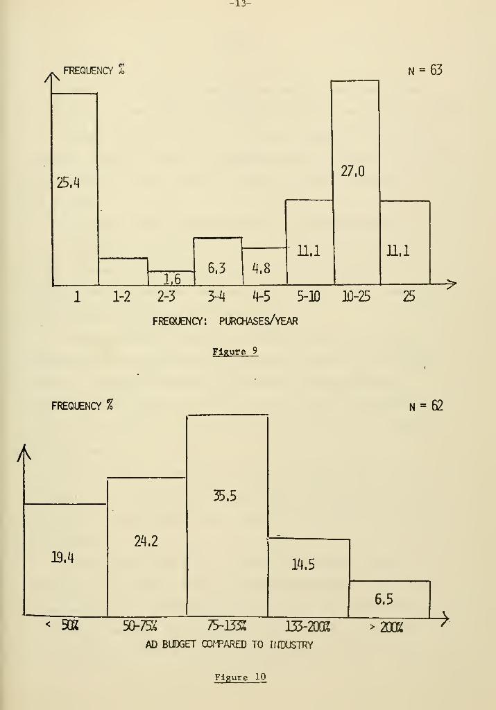
Question 5.6 (Figure 9) considers the average frequency of purchase

by average customers. The distribution of purchase frequency is bimodal,

with one group of products purchased monthly or more frequently and another

less frequently than one/year.

Question 5.7 refers to the number of competitors for the product.

The average number is 13 and ranges from to 1050.

Question 5.9 is a measure of seller concentration. If we sum the

market shares of the three market leaders, the average value is 178, and

the range is from .13 to 1.0.

Question 6.1 gives the total amount spent on selling expense for

these products. The average amount is $3.2 million, (median is $768,000)

and varies from $5,000 to $37 million.

Question 6.3 shows that the largest average element in 1973 ad bud-

gets was Trade and Technical Press with an average of 41% of the ad dollar.

Question 6.5 (Figure 10) compares the product ad budget to industry

average. As the associated figure indicates, ad managers perceive that

their products get a bit less than industry average, but the distribution

is quite varied.

Question 6.6 considers personal selling and technical service expenses,

the means of which are $1.1 million and $530,000 respectively.

-13-

/^FREQUENCY I

25A

lA6.3 ^.8

U.l

N = 63

27.0

1-2 2-3 5-4 4-5 5-10 ]D-25

FREQUENCY: PURCHASES/YEAR

25

Figure 9

FREQUENCY %

y^

19.4

24.2

< SOK

35.5

14.5

N = 62

6.5

50-75X 7^-1332 133-20(K

AD BUDGET CO^PAR£D TO IfffiUSTRY

>2002 ^

Figure 1

-14-

Questlon 6.9 (Figure 11) considers the number of salesmen selling

the product. The mean number is 685 (medlan=30) with a range from 1 to 6000.

Question 6.10, the fraction of an average salesman's time, when mul-

tiplied by Question 6.9 gives the effective number of salesmen. So Question

6.10 * Question 6.9 has a mean of 122 (median of 10) and a range from

.13 to 1440.

The answers to some questions have not been discussed here. This

is for two reasons: first, as the average of the entries is available

in the appendix, discussion here would be redundant. Secondly, some

variables make the most sense when combined with others. Some composite

or constructed variables are considered below.

Consider three key variables, advertising, marketing and sales.

Advertising is the sum of Direct plus Allowance amounts for 1973 in Ques-

tion 6.2. Marketing is defined as Advertising + Personal Selling +

Technical Service, where the latter two items are found in Question 6.6.

Sales is the average price per unit times the niomber of units or Question

3.1 times Question 4.1

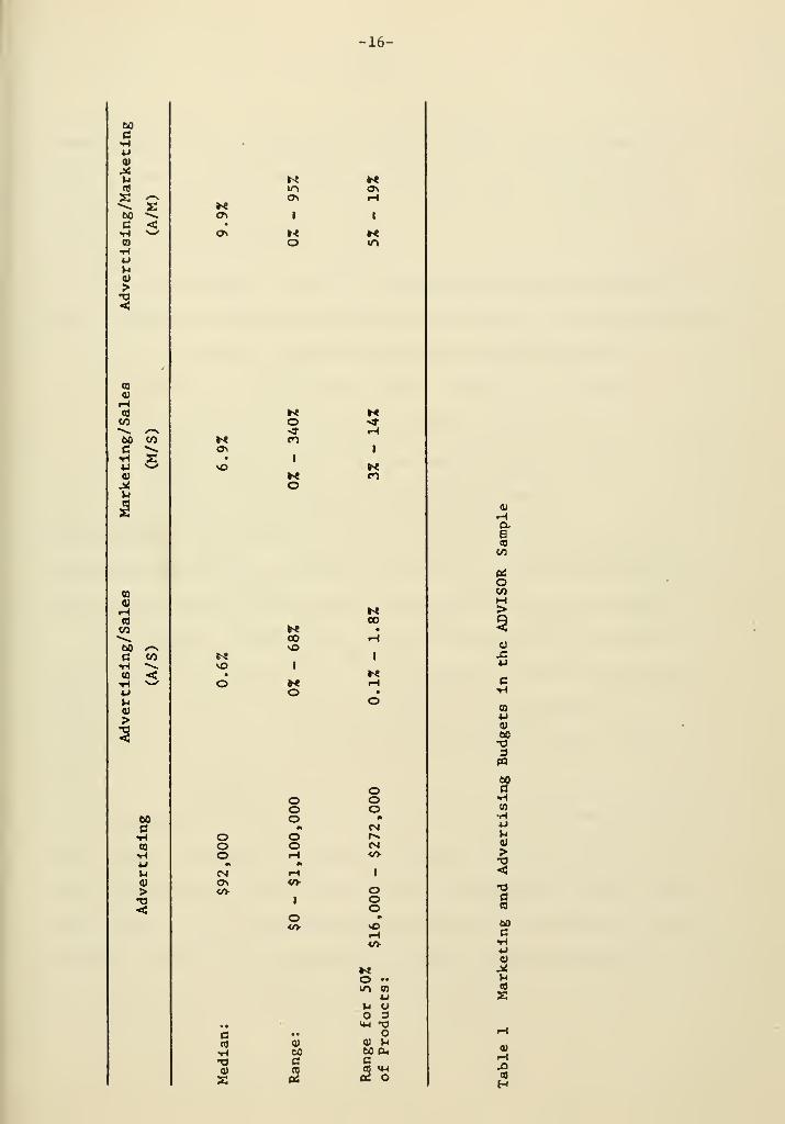
Characteristics of the budgetary data are given in Table 1, and

discussed below. The median advertising budget for the products sampled

is $92,000 and the ad budget midrange (middle 50% of products) is $16,000

to $272,000.

A more important variable is the ratio of advertising expense to

sales (A/S). The median A/S ratio is 0.6%, which is small. This clearly

demonstrates that marketing communication is not a major item in indus-

trial product expenditures, although we believe it to be important in

the marketing mix. The A/S range, however, is wide, 0% to 68%. The latter

-15-

•

-16-

00

uCO

c

-17-

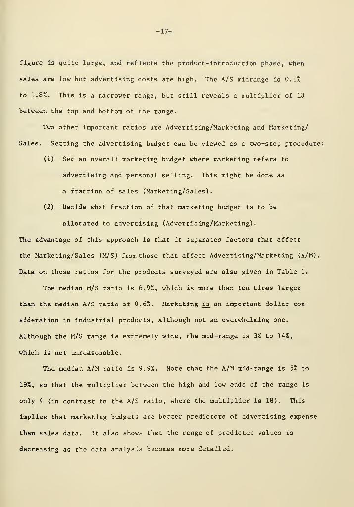
figure is quite large, and reflects the product-introduction phase, when

sales are low but advertising costs are high. The A/S midrange is 0.1%

to 1.8%. This is a narrower range, but still reveals a multiplier of 18

between the top and bottom of the range.

Two other important ratios are Advertising/Marketing and Marketing/

Sales. Setting the advertising budget can be viewed as a two-step procedure:

(1) Set an overall marketing budget where marketing refers to

advertising and personal selling. This might be done as

a fraction of sales (Marketing/Sales).

(2) Decide what fraction of that marketing budget is to be

allocated to advertising (Advertising/Marketing).

The advantage of this approach is that it separates factors that affect

the Marketing/ Sales (M/S) from those that affect Advertising/Marketing (A/M)

.

Data on these ratios for the products surveyed are also given in Table 1.

The median M/S ratio is 6.9%, which is more than ten times larger

than the median A/S ratio of 0.6%. Marketing is an important dollar con-

sideration in industrial products, although not an overwhelming one.

Although the M/S range is extremely wide, the mid-range is 3% to 14%,

which is not unreasonable.

The median A/M ratio is 9.9%. Note that the A/M mid-range is 5% to

19%, 80 that the multiplier between the high and low ends of the range is

only 4 (in contrast to the A/S ratio, where the multiplier is 18). This

implies that marketing budgets are better predictors of advertising expense

than sales data. It also shows that the range of predicted values is

decreasing as the data analysis becomes more detailed.

-18-

The results presented thus far, although simple, have yielded valuable

information: they have already provided rough percentage guidelines for

advertising budgets. As an important further benefit, they have also done

the same for marketing budgets (e.g. 6.9% of sales is not a bad start for

a marketing budget). But the key issue is to relate product-market-custoraer

factors to the budgetary figures.

5. Data Reduction and Analysis

If one adds up all the blanks available for data entry on the question-

naire, one will find 190 "variables". It is desirable to pare down this

extensive set of information for at least two reasons: (1) many fewer than

190 independent characteristics are represented by these variables, and

(2) for any model to be meaningful it must contain as few variables and

be as simple as possible to be understood and used by managers.

Almost half the data come from Section 5. An initial attempt at

variable collapsing started here and was later extended to the questionnaire

as a whole.

The first step was to logically collapse most of the variables into a

smaller set, without losing too much information. The method used is illus-

trated for Question 5.4.

Question 5.4 of the questionnaire asks how routine the purchase decision

is for purchasers. If we assume these data are roughly interval scaled we

PD = 4*Q5,4a + 3*Q5.4b + 2*Q5.4c + Q5.4d

-19-

A high score on PD (near the maximum of four) Indicates that a routine

decision is made "on the average" by the purchasers in deciding to buy the

product. A low score (near the minimum of one) represents a decision which

"on the average" is made at a high level in the company. Other variables

were constructed in a similar fashion.

Table 2 summarizes the first reduction of variables, in Section 5,

from 84 to 25. An initial attempt was made to factor analyze these data,

without success. Because of the ordinal and highly skewed nature of these

data, this lack of success was not surprising. (see Rummel [8]).

Aggregative hierarchical clustering was then used to locate groups

of similar variables. A measure of association or similarity between vari-

ables was selected. Gamma (y) , was used, defined as the difference between the

observed proportion of concordant pairs (given no ties) and the observed pro-

portion of discordant pairs (also given no ties). (see Kruskal [3])

The gamma statistic takes on values between +1.0 and -1.0.

Another candidate for measure of association is the product-moment

correlation coefficient. However, with these badly skewed marginal distri-

butions, the maximum and minimum values of r vary greatly. (see Ritter [7

]

for a discussion of limiting values of r in the case of skewed marginal

distributions.) The product-moment correlation was compared with Y and was

seen to be unstable as suspected.

Ritter [7] gives a complete listing of the matrix of gammas used for

clustering. These clusters can be represented pictorially by a dendrogram

or tree structure as in Figure 12. The numbers running down the left side

of the Figure is the level of association (gamma, here). The branches of

the tree join at levels which represent the measure of association for the

-20-

Table 2

Variables for Input to Clustering

Variable Description

V60-V67 Number of users/resellers for product/industry in 1973/1972

YV Score indicating geographic spread of product volume(high score = widespread)

YC Score indicating geographic spread of product customers(high score = widespread)

IV Score indicating geographic spread of industry volume(high score = widespread)

IC Score indicating geographic spread of industry customers(high score = widespread)

V104 Fraction of product sales to three largest customers

V105 Fraction of industry sales to three largest customers

PD Score indicating how routine purchase decision is

(high score = routine)

V117 Average number of people influencing decision to buyfor largest third of customers

V125 Number of competitors in 1972

V126 Number of competitors in 1973

V127 Number of competitors entering industry since 1969

V128 Number of competitors leaving industry since 1969

MS2 Market share of three market leaders in 1972

MS3 Market share of three market leaders in 1973

V137 Largest change in market share 1971-1973

SW Score indicating ease of switching to competitiveproduct (high score = difficult to switch)

BD Score indicating frequency of buying decision(low score = frequent decision)

CM in CO o%

-22-

cluster. The score for the cluster appears near the point at which the lines

join. (Everltt [ 2] provides a summary of cluster analysis methods).

Figure 12 presents the results of the cluster analysis for this sec-

tion of the questionnaire. The two horizontal lines indicate levels of

association corresponding to gamnaequal to .6 and .9. These lines Indicate:

(1) All of the clusters which join at gamma greater than .9 are clusters

(pairs) of variables representing 1972 and 1973 values of the same

attribute. Further, there are no 1972/1973 variable pairs included in

the analysis which do not associate this way.

(2) Of the six clusters which form at gamma between .6 and .9, five of

them are clusters of responses for product and industry on the same

attribute. There are no other product/industry variables pairs which

do not join in this region.

The first pattern might have been anticipated, but the second one is

not that clear. At least two interpretations of this result are possible.

First, the completer of the questionnaire may have little knowledge of the

"real" answers to the questions for the industry and guesses at an answer

which is like the answer for the product. Or perhaps, because most of the

sample is from products which are considered market leaders, what is true

for the product is true for the industry because in some sense the product

is the industry. These two explanations may interact: perhaps the product

manager has no real knowledge of the industry answers, but feel confident

in assuming that industry practices are similar to the product because the

product is a market leader.

Finally, note that no other pairs of variables are as closely related

(statistically) as the 72-7J and company-Industry data.

-23-

This procedure was repeated in other sections of the questionnaire and

with other clustering rules. In all cases the same basic results held,

leading to the following conclusions.

(1) Company and industry data are not sufficiently distinguished to

Justify inclusion of both in model development.

(2) Data do not change enough between 1972 and 1973 to include direct

variables from both years in any model. Thus we will choose

1973 for consistency, but we still may wish to consider year to

year changes in variable levels (1973 customers - 1972 customers,

say).

To develop a rationale for identifying related variables, consider the

following: transform each of the potential independent variables into dicho-

tomous variables (High/Low) by splitting the sample at the median. Do the

same for Advertising/Sales, Advertising/Marketing and Marketing/Sales. Now

crosstabulate the variables and see which variables seem related. Splitting

these samples at the median stabilizes the analysis by reducing the effect

of outlying points.

As an example, consider Figure 13.

Growth Rate (Q4.3)

AdvertisingSales

21

-m-

Table 3

Y-Coefficlents of 2x2 Cross-Tabulations

IndependentVariables*

Advertis-ing/Sales

MktgSales

Ad

_Mktjs_

1. V020 Stage in Life Cycle

2. V058 Plant Utilization

3. V059 Industry Lead Time

k. PRICE Price5. INCR Incremental Margin

6. CPR Customer Perception of Price

7. MSR Market Share8. GRO Growth Rate

9. IGRO Industry Growth Rate

10. CHANT Distribution Channels

11. II Quality-Distinguishability

12.

13.

14.

15.

16.

17.

18.

19.

20.

21.

22.

23.

12 Total Gross Margin

14 Industry Profit Index

IB Customers Growth Rate

1106 Company Total Sales

1108 Price Elasticity

1109 Total Net Margin

1110 User Perception of Price

1111 Reseller Perception of Price

1112 Change in Market Share

1114 Number of Customers

1115 Your Customer Concentration

1116 Industry Customer Concentra-

tion

24.CUSCON Sales to 3 largest customers

25. INCON Ind*. Sales to 3 largest

customers

26. IMPORT Purchase Import

27.NOCOMP Number of Competitors

28. MLDR Share of Market

29. MSDEL Change in Market Share

30. SWIT Ease of Switching

31. SELL Selling Expenses

32.SELIND Selling + TS Exp.

33. NOMAN Number of Salesmen

RM Effective no. of Salesmen

19 Frequency of Purchase

110 Sales/Customer

111 No. of Deciders

113 <f Competitors In + Out

115 Dollar Sales

34.

35.

36.

37.

38.

39.

.70

.23-.03

-.32

.21-.09

-.45

.49-.09

.15

.42

.36-.3

.15

.21

.03

-.2

.03-.33

-.32

.45

.04

.16

-.32

-.03

.02

-.09

.49

.16

.03

.66

-25-

Here annual volume growth rate is compared to Advertising/Sales; a positive

relationship seems to exist. The measure of the degree of association seen

here also is the y coefficient mentioned above. Table 3 details a long list

of associations. The definitions of those variables are found in Appendix 2.

There are several important points to note from Table 3. First, the

variables are dependent on one another in varying degrees. Thus, as noted

earlier, the number of variables must be reduced. The sample size (66)

compared to the number of variables also necessitates this reduction. The

analysis above indicates that we will not be able to further cluster the

variables statistically; therefore we shall classify variables into cate-

gories which are logically independent of one-another.

The second point to note is that if we let Advertising = A, Marketing

= M, Sales = S; then A/S E A/M • M/S. Now, note the patterns of association

In Table 4.

Because of the association noted above between A/S, M/S, A/M, the

ratios can be closely related to an independent variable in one of several

ways. Let represent a weak or non-existent relationship, (^ strong relation-

ships, either positive or negative, and <'-^ strong relationships in the oppo-

site direction. Then, Table 3 reveals the following patterns of association:

Table 4: Association Patterns in Table 3

Pattern

-26-

Patterns 1 and 2, in Table 4, suggest that A/S can be related to an

Independent variable either if one of the other ratios or both of the other

ratios are related. Patterns 3 and 4 suggest that no relationship may exist

for A/S either if no relationship exists among the other patterns or if

conflicting relationships exist.

Looking down the first few variables in Table 3, Stage in Life Cycle

is an example of pattern 1, Plant Utilization is an example of pattern 2,

Industry Lead Time, pattern 4 and Customer Perception of Price, pattern 3.

All variables do not, of course, fit neatly into this type of package.

But enough do to suggest that a meaningful relationship between A/S and

independent variables might be derived if a two-step procedure is used; model

A/M and M/S separately and combine the results to form A/S.

In the next section we compare several methods of modeling the A/S

ratio. Before proceeding, we classify the important independent variables,

those closely associated with the ratios of interest here, into categories

in Table 5.

Table 5: Main Variable Categories

1. Stage in Life Cycle

2. Product Perception

3. Growth Rate

4. Frequency, Quantity Purchased

5. Buyer Concentration

6. Compmy Position, Market Share

7. Plan_ Utilization

8. Prici-, Margin

-27-

The above variable-categories may still not be independent. However, such

a set of variables forms a good list to use for development of a model; a

more detailed look at construction of composite variables in these cate-

gories together with an associated correlation or association matrix may

call for still further reduction. However, the Table 5 list, both logi-

cally and statistically, appears to be a good starting point for analysis.

6. Advertising Budgeting Guidelines

Consider the following possible procedure for setting the ad budget:

Ad manager X collects the data requested in the project questionnaire. He

then uses that information as follows:

"Product XYZ has 873 customers and we budget 1% of sales for

every 10,000 customers so we add .087% of sales as a customer

effect; our plant utilization is only 60% leaving 40% unused capacity,

we add .125% for each 10% of unused capacity, so we add .5% of sales,...," et(

Our product manager then adds up all these quantities: .008 + .005 + ...,

etc. to get an advertising/sales ratio as a proposed budgeting figure. Thus

he has a checklist of items; and he takes each item into account separately

while computing an advertising budget.

A mathematical model which this form of budget developments suggests

is as follows:

(1) A/S = k_ + k -No. customers -- k. • unused capacity + ..., etc.

According to the scenario above k = .001, k_ = .125, etc. This form

of model was tried, both as in (1) and in a multiplicative form with consis-

tently poor results as follows:

-28-

(1) The models did not fit well, particularly at the extremes.

(2) The effects of several variables were in the, wrong logical direction.

(3) Small changes in the model form (adding or deleting variables) changed

the coefficients significantly.

The reasons for the poor fit seemed to be the following:

(1) The data have wide ranges and some distributions are highly skewed.

(2) More than one budgeting process may be represented in the sample.

(3) Actual budgeting processes may use much less well-defined data.

Resolving the issues implied in (1) and (2) is a difficult job. To-

gether they imply that a variety of submodels should be developed for vari-

ous ranges of the Independent variables. But in what ranges? And how many

submodels?

An insight relative to point (3) may go a long way toward satisfying

points (1) and (2), During unstructured Interviews with ad managers, the

reasons for budgeting high for advertising were such statements as"large

number of customers," "early in life cycle"; much unused plant capacity...",

etc. No explicitly quantitative guidelines ever arose.

Thus, if ad managers think in terms like High vs. Low, Early vs. Late,

etc., a model which treats variables continuously as in Equation (1) may

be trying to extract more information about the decision process than is

actually there. In addition, as most ad managers had difficulty obtaining

some of the information on the questionnaire, that information may not be

readily available in the quantitative form asked for.

The above discussion suggests dichotomizing the continuous (and multi-

leveled discrete) independent variables into High and Low categories for

-29-

purposes of building a model. It also suggests that the output shoikld per-

haps be in a High vs. Low, or, at best, a High, Medium, Low form.

How should High and Low categories be constructed? In some cases, the

answer is unambiguous — Stages 1 and 2 of the life cycle are "early"; 3

and 4 are "late". In most cases, however, there is no logical break-point

and the sample median is used.

In this framework the decision-maker is considered to have a check-list

of product/market/environmental characteristics relevant to the budget deci-

sion. The values of the characteristics are only known roughly (HIGH versus

LOW, say). The decision maker then considers these characteristics one at

a time , with the value of each characteristic adding or subtracting some

value from the final budget score.

Finally, the guidance that the budgeter gets from the checklist is not

only a given budget amount, but rather a range of amounts. He is thus told

that the budget for this particular product should be low (<l/3% of sales,

say) consistent with industry norms. Figure 13 illustrates the procedure

conceptually. One takes a particular product through the checklist and

gets guidance on whether that product's ad budget should be High, Medium or

Low.

Until now we have treated advertising budgeting as if it were a one-

Step procedure. However, as noted before, analysis of the associations

suggests that the process, both conceptually and logically, might be thought

of In two steps, first setting Marketing/Sales then Advertising/Marketing.

The advertising budget could then be viewed as

, , Advertising Marketing „ ,Advertising = —r^

—

.——; °- • —r—; °-

• Sales° Marketing Sales

The conceptually satisfying aspect of modeling the budgeting process in this

-30-

Factor

Life Cycle

Plant Capacity

Number of

Customers

Level Ad Budget

FIGURE U Conceptual Framevork of the Budgeting Proeea g

-31-

two-step way is that some variables tend naturally to be associated with

A/M; others with M/S; still others with both. Modeling the procedure in

two steps gives Insight into the determinants of the separate processes

whereas the single step process may mask important information. In the

final analysis, any procedure must classify accurately; the classification

ability of the one-step and two-step procedures are explored below.

The discussion above Indicates that it is desirable to be able to

classify A/S, M/S, and A/M into categories (high-low or high-medium-low).

This objective suggests that discriminant analysis might be considered as

a means of estimating the function of independent variables which best

separates the (already classified) dependent variables.

A variety of discriminant analyses were run, using 2 group and 3 group

classifications (Groups were developed empirically so that the break point

between "High" and "Medium" A/S, say, occurs at the least of the highest

1/3 of the sample A/S ratios). The independent variables included variables

from the categories suggested in Table 5.

The discriminant analyses gave reasonably good fits; but, they all

suffered from unstable coefficients (small changes in data lead to large

changes in coefficients). On the other hand, regression analysis, as per-

formed below, provided results just as good in classification and prediction

with more stable coefficients. Regression was, therefore, selected over

discriminant analysis as the method for further development. The objectives

of the regression analyses were basically the same as those of the discrimi-

nant analyses.

Regression analyses were originally run, estimating A/S, M/S and M/S

as functions of the variables from Table 4. Use of the actual ratio data

-32-

led to unstable coefficients as would be expected from the skewed distribu-

tions of the dependent variables. Regressions were also run against the

medians of the three sets of three classification groups. This approach

worked well, but not quite so well as the approach described below.

In order to stabilize the skewed A/M, A/S, M/S distributions, new

variables called RANKAM, RANKAS, RANKMS were defined be transforming the

original A/M, A/S, and M/S. RANKAS is an empirical normalized rank trans-

formation of A/S as follows: RANKAS- empirical rank/It of non-tied points.

Suppose there were four points in the sample: .0010, .00014, .0010, .0020.

These would be transformed to 1/3, 2/3, 1/3, 1 respectively. The ranks

then must be translated in a useable ratio.

The purpose of this transformation is to stabilize the A/S, A/M, M/S

ratios so that their long right-hand tails do not overwhelmingly affect para-

meter estimation. Ties are given equal numbers, and no ranks are left blank.

The best models and variables (in terms of logical development and

statistical stabilitj^ are detailed in Table 6, the definitions of variables

in Table 7.

-33-

TABLE 6: RANK MODELS

RANKAS -

RANKAM

-.074

-34-

TABLE 7: VARIABLES IN MODELS

1. RANKAS - Normalized Advertising to Sales Rank, ranging from to 1.

2. RANKAM " Normalized Advertising to Marketing rank.

3. RANKMS - Normalized Miirketlng to Sales Rank.

4. LIFECYCLE = Product stage in life cycle, ranging from 1 to 4. Q 2.8 of

questionnaire.

5. FREQ Indicator variable constructed from Q6.5 as follows:

NT - 50 *Q5.6a + 20 * Q5.6b + 4 * Q5.6c + Q5.6d + 1/4 * Q5.6e

+ 1/10 * Q5.6f

and FREQ - /'I IF NT > 4.98t ir NT < 4.98

6. ASSOC

7. MSR

8. CUSCON

9. CUSTGROW

" a composite index constructed as follows:

QDA - (Q2.6a + .8Q2.6b + .6Q2.6c + .4Q2.6d + .2Q2.6e)* Q2.2 * Q2.3/16

ASSOC

uIF QDA > .298

IF QDA < .298

{

1 IF Q4.2b > .183

IF Q4.2b < .183

1 IF Q5.3a > .241

IF Q5.3a < .241

an index constructed as follows:

CUST73 = Q5.1 (USERS + RESELLERS 73)

CUST72 = Q5.1 (USERS + RESELLERS 72)

CUGR = (CUST73 - CUST72) /CUST7:

and CUSTGROW .{11(O 1

F CUGR > .006

IF CUGR < .006

-35-

One of the most interesting and surprising of the results is the set

of factors which did not show up as significant. Neither a product category

effect (chemical vs. machinery, say) nor a company-specific effect was

found to be significant in the analysis. This made sense. However, con-

ventional wisdom suggests that some of the following ought to be important:

'Product margin

"Plant utilization

'User perception of price

'Industry profitability

'Number of competitors

'Number of decision-makers in company

'Directness of distribution channels

The non-inclusion of these variables could be due to several reasons —

(a) they are in fact associated but not strongly enough to show up; (b) their

effects are accounted for in combination of other variables or (c) decision

makers in fact do not consider these variables. Further study on a larger

sample would be needed to give insight into these issues.

Table 8 compares these models in an integrated way. The models can

be interpreted by reviewing the columns of Table 8 one at a time.

Stage in Life Cycle . Each product was classified into one of four

stages: Introduction; growth; maturity; and decline. Most managers had

no difficulty classifying their products (although it is remarkable how few

thought their products were in the declining stage). Looking at Table 8

life cycle turned out to have a strong negative impact on the budgeting

ratios. In the M/S ratio entry, the minus sign indicates that as the life

cycle of a product progresses, the value of the M/S ratio decreases (since

-36-

Customer

Growth

-37-

the product becomes established). The A/M ratio is not especially affected,

but on net, the A/S ratio is both strongly and negatively affected. Thus,

early in the life cycle of a product, the Advertising/ Sales ratio tends to

be high; later, it tends to be low.

Frequency of Purchase. Questionnaire data was converted into an average

number of purchases per year. It was rated as high if the frequency was > 5

purchases/year, and as low if < 5. Frequency does not have an appreciable

influence on the M/S ratio, but it does influence the A/M ratio. The more

often the product is purchased, the greater A/M. This is sensible; if

people are purchasing frequently, it may well be worthwhile to send more

messages to them. On net then, purchase frequency has a solid positive

effect on Advertising/Sales.

Product Quality, Uniqueness, and Identification with Company . This is

a composite index made from several questions in the data set. A high score

on this variable would imply that the product had a substantial edge in

quality over its competition, was unique or clearly distinguishable, and

had a strong association with the company name. These factors appeared to

be related, so a composite was constructed that served adequately. This

composite factor had little effect on M/S, but a significant effect on A/M.

If your product has quality, uniqueness, and a strong attachment to the com-

pany name, then you have a story to tell, and you use advertising to do it.

A larger proportion of the marketing budget goes into advertising, and there-

fore, A/S is larger as well.

Market Share . This factor is self-explanatory; a high share was > 18%;

low was < 18%. The higher the market share, the less is M/S. (Of course.

-38-

the absolute marketing budget may be substantial If you are the market leader.

But the M/S ratio tends to decrease with market share.) The A/M ratio is

not strongly affected by market share, but there is, of course, a net effect

on A/S. Again, the higher the market share, the lower the Advertising/Sales

ratio. This is an important finding and indicates that Industrial product

managers behave as if there were economies of scale in marketing that per-

mit decreased expenditures (in a percentage sense) at high shares.

Concentration of Sales . This factor refers to how much of the business

is done with just a few customers. The specific definition is the percent

of product sales purchased by the three largest customers. High was anything

> 2AZ; low was < 24%. As sales concentration increases, the M/S ratio goes

down. (There is only so much you can do with a few customers, so you will

tend to have a smaller marketing budget.) But increasing sales concentration

also increases the A/M ratio, so the net effect on the A/S ratio is small.

Growth of Customers . This factor is the percentage increase in the

number of customers in 1973, as compared with 1972. Again, this is broken

into high (over a 1% increase) and low categories. Customer growth has a

positive effect on the M/S ratio, and interestingly, also on the A/M ratio.

Obviously, the effect on A/S is also positive.

In summary, the factors of stage in life cycle, concentration of sales,

and market share primarily affect the Marketing/Sales ratio. Purchase fre-

quency, and product quality, uniqueness, and identification primarily affect

the Advertising/Marketing ratio. The growth rate in number of customers

affects both ratios slightly. (Note that most factors affect either M/S or

A/M, but not both, confirming our decision to split the A/S ratio Into two

parts.) Putting these effects together generates budget norms.

-39-

The models in Table 6 produce a predicted rank associated with adver-

tising to sales ratio. This has to be translated into a predicted A/S ratio

to see how well the model works. Figures 14 a.b.c relate ranks to ratios

for A/S, A/M, M/S.

Table 9 gives the empirical break points if each of the three ratios

are split into groups of equal number.

TABLE 9 : GROUP BOUNDARIES — 3 GROUPS

Group it

I.

II.

III.

<AS < .0032

.0032 <AS < .017

.017 <AS < 1.0

< AM < .06

,06 < AM < .17

.17 < AM < 1.0

< MS < .05

.05 < MS < .13

.13 < MS < 100

As a test of the model fit. Table 10 gives the actual classification

versus predicted classification for A/S. The fraction properly classified

(the diagonal elements) is 23/45 = 51%. The model predicted group is con-

structed by getting a predicted value for RANKAS, a predicted value for A/S

from Figure 14a and then a classification from Table 9. Data points with

missing values for any independent or dependent variables were eliminated

leaving 45 for analysis and prediction.

TABLE 10 : A/S ACTUAL VERSUS PREDICTED CLASSIFICATION

Actual Group

Model-Predicted

Group

I

II

III

I

o ./ .z *3 '4 'S' '6 n -e* .'^ Ao

.4

3

.Z

.1

,/ .2 .3 .4 '5* .6 '7 /8 '9 /.O

-42-

Now consider A/S as A/S = A/M ' M/S where A/M, M/S are obtained by

estimating RANKAM, RANKMS first from Table 6, theu translating to A/M, M/S

via Figure 14b, c. These figures are then multiplied and their product is

classified into groups from Table 9. In this method 58% (26/45) are cor-

rectly classified, indicating that both the direct and Indirect (A/S »

A/M • M/S) methods yield comparable results. In fact, the samples were

broken at the median, and A/S gave 76% correct classification; while the

direct method gave 75% correct. Thus the methods appear comparable in fit-

ting ability, and are good, though not outstanding. (For comparison, a

random 3-group ranking would be expected to have 33% correct with a standard

deviation of 6%, given our sample size).

A test on data not used for fitting would be desirable. The small

size of the original sample precluded keeping a holdout sample for predic-

tive testing. However, there are a number of data points which have been

excluded because they do not contain all independent variable data.

Seven data points were isolated which were missing at most a single

independent variable on each ratio. The missing variable was assumed equal

to the sample mean for that group and the models were used to classify those

points in both the direct and indirect way. The direct way classified four

of the seven properly; the indirect method, five of the seven. This result

is hardly definitive since the sample is so small but is reassuring in that

the quality is similar to the fitted results.

The overlap in prediction using the two different procedures was com-

pared and the two methods agreed on 65% of the points.

-43-

6. Allocation of the Advertising Budget

The results of the previous section provide guidelines to aid In the

development of an overall advertising budget. A similar analysis shows

how Industry has chosen to allocate those budget dollars among various

media. Four advertising categories were used:

Space: Trade, technical press, and house journals

Direct Mail: Leaflets, brochures, catalogs, and other direct mail

pieces

Shows: Trade shows and industrial films

Promotion: Sales promotion.

The conceptual model of decision-making that is Implied here is simi-

lar to the one described in the previous section: the decision-maker is

viewed as having a checklist of factors (dollar sales, number of customers,

etc.) known only roughly (High-Low); he considers each factor separately,

adding or subtracting each from a final budget score. Table 11 gives the

median budget breakdown in each of the above categories.

In developing relationships between the four categories above and

independent variables, it should be noted that we are modeling four pieces

of a constant sum item (SPACE + SHOWS + MAIL + PROMOTION = 1). Therefore,

we should expect to see a variable which affects one item positively have

a negative relationship with other Items.

The four equations were estimated separately. A more sophisticated

eetimaclon process, constraining the dependent variables to sum to 1, is

possible but would not be likely to Improve the estimation significantly.

Table 12 details the results of estimating parameters of the model.

-A4-

Median Amount

SPACE 41Z

SALES PROMOTION 2AZ

DIRECT MAIL 2AZ

TRADE SHOWS, EXHIBITIONS IIZ

Table 11 Allocation of the Advertising Budget

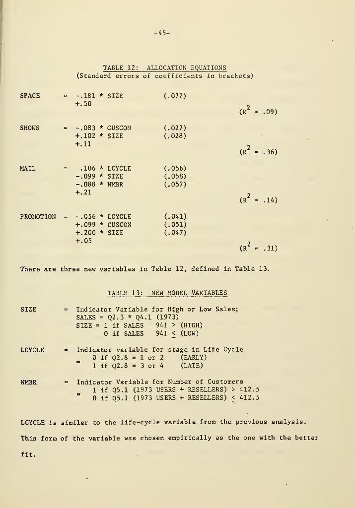
-45-

TABLE 12: ALLOCATION EQUATIONS(Standard errors of coefficients in brackets)

SPACE

SHOWS

MAIL

PROMOTION =

-.181 * SIZE+.50

-.083 * CUSCON+.102 * SIZE+.11

.106 * LCYCLE-.099 * SIZE-.088 * NMBR+.21

-.056 * LCYCLE+.099 * CUSCON+.200 * SIZE+.05

(.077)

(.027)

(.028)

(.056)

(.058)

(.057)

(.041)

(.051)

(.047)

(R^ .09)

(R^ ,36)

(R .14)

(R^ .31)

There are three new variables in Table 12, defined in Table 13.

SIZE

LCYCLE

NMBR

TABLE 13; NEW MODEL VARIABLES

Indicator Variable for High or Low Sales;

SALES = Q2.3 * Q4.1 (1973)

SIZE = 1 if SALES 941 > (HIGH)

if SALES 941 < (LOW)

Indicator variable for stage in Life Cycle

if Q2.8 = 1 or 2 (EARLY)

1 if Q2.8 = 3 or 4 (LATE)

Indicator Variable for Number of Customers

1 if Q5.1 (197 3 USERS + RESELLERS) > 412.5

if Q5.1 (1973 USERS + RESELLERS) < 412.5

LCYCLE is similar to the life-cycle variable from the previous analysis.

This form of the variable was chosen empirically as the one with the better

fit.

-46-

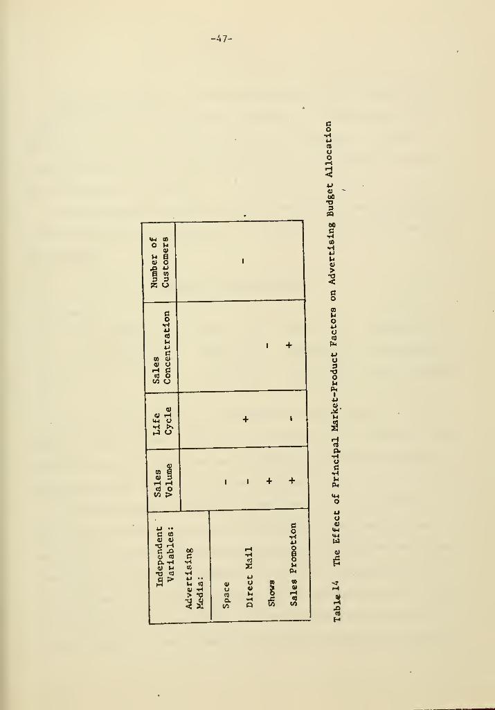
Table 14 summarizes the results of these equations. The Impact of

the important factors on the various advertising media is briefly described

below. Two of the factors, sales concentration and number of customers,

are highly correlated and were not jointly used in any one analysis.

Sales Volume . Sales volume is negatively related to direct mail

advertising, perhaps owing to saturation effects. The relationship for

shows and promotion is positive, possibly indicating that as sales goes

up, newer forms of communications are sought. The relationship with space

media is very weak and slightly negative — larger sales reduce the frac-

tion of space advertising. None of the factors had a strong effect on

space. Our interpretation is that space advertising is a rather constant

fraction of advertising budgets (about 41% in our sample), and is not

greatly affected by product and market characteristics. But with a larger

sales volume, more money is available for other forms of advertising.

Thus, a slight negative relationship emerges for space.

Stage in Life Cycle . Products late in the life cycle spend propor-

tionally more on direct mail advertising. (Customers are likely to be

better known, and few new customers are sought.) There is little effect

on shows. On promotion, the effect tends to be negative; i.e.. early in

the cycle, greater effort is made in sales promotion. Later on, effort is

transferred, percentagewise at least, to other forms of advertising.

Concentration of Sales . Sales concentration is negatively related

to shows ~ if you have few customers, trade shows are a poor way to reach

them. In contrast, a lot of effort will be put into sales promotion, and

as expected, the relationship between sales concentration and promotion is

positive.

-47-

§U9Uo

<M

-48-

Number of Customers . If you have many customers, you are less likely

to use direct mail advertising, since other forms of communication may be

more efficient. The factor does not appear in the analyses of the other

advertising media since its complementary factor (concentration of sales)

was felt to be more appropriate.

As in the budget allocation model these models were used to classify

media fractions in High, Medium and Low categories. Table 15 lists empirical

break-points.

TABLE 15: GROUP BOUNDARIES

GROUP //

I SPACE > .41

II SPACE < .41

MAIL > .30

.30>MAIL>.15

.15 > MAIL

SHOWS > .15

,15>SHOWS>.05

.05 > SHOWS

PROMOTION > .29

.29>PROMOTION>.06

.06 > PROMOTION

Note that only two groups are included for SPACE. This is necessary

since the SPACE equation includes only one variable and it is binary. There-

fore, only two prediction values can be derived from the equation making a

three category (HI, MED, LO) prediction fruitless.

That the fractions properly classified were 74% for Mail, 67% for

Shows, 55% for Promotion and 34/55 =» 62% for Space. These should be com-

pared with an expected random classification accuracy of 33% for three group

classification (MAIL, SHOWS, PROMOTION) and 50% for two groups (SPACE).

Once again, a truly predictive test in data not used for fitting would

be desirable for evaluating models. A holdout sample was not used due to

the small sample size, but a number of data points were available for MAIL,

-A9-

SHOWS and PROMDTION which excluded one bit of independent variable data.

The model for MAIL classified 4 of 6 data points correctly, the model for

OTHER 4 of 6 and that of SHOWS 3 of 5.

7. Use

The results of the ADVISOR project provide new forms of guidelines

for industrial marketing management, both for setting an advertising budget

and dividing that budget among media.

An interactive computer program was developed for the project partici-

pants. The program allows operation of the model in the user's office via

a remote terminal. The program asks the user relevant questions from a

reduced form of the project questionnaire. The program translates these

values into high or low rankings, depending on the breakpoints developed

from the data base. These rankings then go into the model, which produces

budgeting and allocation guidelines (not just a fixed number, but also the

range of most common values).

The product manager is the mediator in this process. He gathers the

Input, puts it into ADVISOR, and gets back the guidelines. He then makes

his recommendations as he sees fit, considering all the information at his

disposal. ADVISOR does not tell him what he should do, only what the

typical industry response would be, as represented by the ADVISOR sample.

The program and model allow several uses including

'Establishing spending levels for new product advertising

'Allocating budgets in multi-product lines

'Projecting marketing costs for budgetary planning

-50-

* Studying complex changes in marketing variables

'Exception reporting — discovering situations where budget reviewis needed.

'Product analysis — discovering situations where special factorsexist, or where managerial conception of a product is inaccurate.

For more details on methods of using the results eee Lilien and Little [ 5 ]

8. Further Work

The ADVISOR study breaks new ground in providing empirical support for

Industrial marketing decision-making. There is no claim that these results

are a "final" answer. The data base was small, as was the number of companies.

In addition, no study of practice can develop iJesults which can unambiguously

be adopted for use — users must be convinced that industry's collective

wisdom is valle for their particular problem.

Thus, there are several alternatives for further work in this area.

One would be to extend the data base to test and improve the models developed.

Many of the results would be more definitive if confirmed on a larger sample.

A larger data base would also allow testing for several factors that are

currently not significant.

Another direction for future work is to study explicitly what industrial

marketers should do, even if they are not doing it now. Fewer products would

be used in such a study, but much more detailed analysis would be performed.

Time-series data would be collected to alleviate some cause-and-ef feet diffi-

culties that are always present in purely cross-sectional studies. Some

-51-

experimentation, either controlled or natural, could strengthen results.

Both these research directions are now being pursued in a follow-up

study, ADVISOR 2, which promises deeper insight into the budgeting process,

and more powerful tools to aid industrial marketing managers.

-52-

REFERENCES

1. Bowman, E. H., "Consistency and Optimality in Managerial Decision-Making," Management_Science, Vol. 9 (January 1963).

2. Everitt, Brian. Cluster Analysis . New York: Wiley & Sons, 1974.

3. Kruskal, William H., "Measures of Association for Cross-Classifications,"Journal of the American Statistical Association , Vol. ^t9 , No. 268

(December 1954) .

4. Kunreuther, Howard, "Extensions of Bowman's Theory of ManagerialDecision-Making," Management Science , Vol. 15 (April 1969).

5. Lilien, Gary L. and John D. C. Little, "The ADVISOR Project: A Study

of Industrial Marketing Budgets," Sloan Management Review (Spring 1976).

6. Lilien, Gary L. et al. , "Industrial Advertising Effects and Budgeting

Practices," Journal of Marketing , Vol. 40, No. 1 (January 1976).

7. Ritter, M. A., "Identifying Clusters of Variables in the ADVISOR

Questionnaire," Unpublished SSM-MIT Research Report, May 1975.

8. Rummel, R. J. Applied Factor Analysis . Evans ton, IL: Northwestern

University Press, 1970.

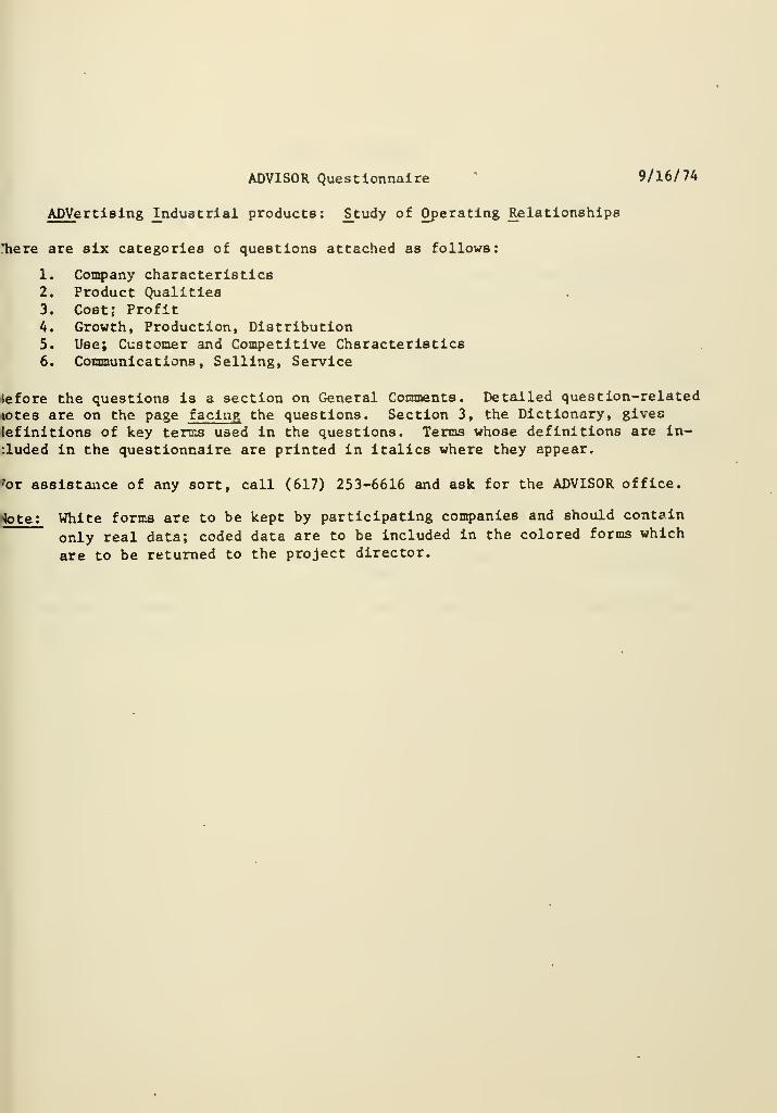
ADVISOR Questionnaire * 9/16/74

ADVertlsing Industrial products: S^tudy of Operating Relationships

liere are six categories of questions attached as follows:

1. Company characteristics2. Product Qualities3. Costj ProfitA. Growth, Production, Distribution5. Use; Customer and Competitive Characteristics6. Communications, Selling, Service

tefore the questions is a section on General Comments. Detailed question-related

lotes are on the page facing the questions. Section 3, the Dictionary, gives

lefinitions of key terms used in the questions. Terms whose definitions are in-iluded in the questionnaire are printed in italics where they appear.

'or assistance of any sort, call (617) 253-6616 and ask for the ADVISOR office.

tote: White forma are to be kept by participating companies and should contain

only real data; coded data are to be included in the colored forms which

are to be returned to the project director.

-2-

GENERAL COMMENTS

1. All proportions are asked for as fractions here: thus a 15Z market-shareshould be entered as .15.

2. When there is doubt about how to define a quantity that is not specified inthe DICTIONARY, use the operational definition in use in your company. Besure that definition is used consistently throughout your company's ques-tionnaire responses.

3. Most quantitative questions allow for considerable answer tolerance (+ 10%for example). Before spending much effort digging for more accurate answers,first see if answers are easily available to the degree of accuracy requested.

4. Questions marked with a star (*) are those for which a coropany-security-factor(CSF) should be used to multiply results. See the notice on Security Proceduresfor more details.

5. One can usually distinguish between three types of data: hard, soft and noinformation. Thus, soft data (one's best guess), while not to be preferredto "hard", is much more desirable than "no information."

6. Where there is no decimal point incltjded in an answer category, right-justifyall answers, (e.g. , 10 in should be i 0) •

7. Numbers in parentheses, (35-41) e.g., are key-punching instructions and canbe ignored during form completion.

-3-

SPECIFIC NOTES

1.2 If a company wishes to consider more than one of its operating divisions asseparate Units then it should enter an identification number of its choicein the space labelled "Unit I.D.".

If classification is clear, enter the correct code in space(4) ; ifdoubtful, completion of B is recommended.

Some "products are very closely associated with the parent company (e.g.,Kellogg'

8

Corn Flakes), others are less closely associated. A productwhich is closely associated with the company may receive an "umbrellaeffect" from the company's reputation which may be reflected in itsselling budget.

An image leader is a product which could be considered to be "carrying"the company mame. To do this Job, the company might spend proportionallymore on communications. At the other extreme, a product to be phased outmight find the company spending considerably less on communications thanone might expect.

-4-

" 1. Conpany Characteristics S 1 (1-2)

• Company I.D. (A-5)

IUnit I.D. (if any) ~ ~

(7_8)

IProduct I.D. .

~ ~ (10-13)

.1.1 What were total company-unit dollar sales (in million $) 1972: ._ (14-19)

I1973: ._ (21-26)

1.2 What were total (before tax) unit profits? (in million $) 1972:.

(28-33)

j

1973:.

(35-40)

2. Product Qualities§L 1 (1-2)

2.1 Which of the following categories, in your opinion, best describesthe product? Complete A or B.

A. 1 » Machinery and Equipment2 = Raw Material, other than chemical3 = Fabricated material (glass, plastic, etc.)4 = Component part5 = Salvage good6 " Chemical7 = Service8 - Other (Describe) (4)

B. Give SIC Code (6-9)

2.2 Is product generally regarded as

1 « Not distinguishable from industry '

3

2 = Somewhat different3 = Very different4 = Unique _ (11)

2.3 How closely related do you feel the product is with the company

In the minds of your customers?

1 = Not at all2 = Just a little3 = Somewhat4 «= Highly _ (13)

2.4 Is this product

1 - Produced to order2 - Standard, carried in Inventory _ (15)

2.5 Does the company regard this product as

1 - An image leader

2 - Fairly important

3 - Average in importance

4 Below average in Importance

5 » A product to be phased out , _ (17)

-5-

Note that pvoduat quality or performance, separate from price.Is requested here. If you feel that half your cuetomers per-ceive your product to be "somewhat better" and the other halfto be "about the same", then enter 0.5 in categories b and cand 0.0 elsewhere.

The stages of the life cycle can be defined as follows: DuringIntroduction , the sales of the product (industry) rise slowly;if it "catches on," there is a period of rapid Growth in salesvolume; this fs followed by a longer stage of Maturity in which6ales grow slowly or are stable; finally there is a stage of pro-longed or rapid sales Decline . Industry here means an impression ofan average competitive product.

Gross margin is defined as (total revenue - total cost)/ number of unitesold in the year in question. This does not include advertising, selling oroverhead. If revenue were $2 million, cost $1.5 million, and 1 millionunits were sold, gross margin would be % .bOlunit. Price (question 3.1)

would be $1.50/unit and gross margin as a fraction of price would be .50/1, 5i

- .33.

If you had a single competitor with a market share of .60 and his marginwas 1.7 times your own, you would enter .60 in line a and .40 in linec (representing your prof it ). Lines a, b, c can be interpreted "higher

than yours," "about the same," "lower than yours" if quantitative infor-

mation is not available.

In the example in 3.3, assume revenues were to increase by $.2 million

(2.0 to 2.2 million), variable cost from $1.5 million to 1.6 million.

Then the number requested is (2.2 - 2.0)/(1.6 - 1.5) - 2.0. This numbermay, of course, be negative in certain cases.

-6-

I How do you think your customers perceive your product quality

relative to industry average? (Enter the corresponding frac-

tion of relevant customers in each line.)

a. Substantially superior *_. (19-21)

b. Somewhat better _• (23-25)

c. About the same _. (27-29)

d. Somewhat poorer _• (31-33)

e. Substantially poorer _• (35-37)

Total=1.0

,7 Have there been any major technological changes in this

industry since 1969? If in doubt, enter 2^.

Yes - 1

No - 2 _ (39)

:.8 At what stage in its life cycle would you say the product

and the industry are in?

Introduction Growth Maturity Decline

Product =1 -2 =3 -4 _ (41)

Industry =1 =2 =3 =4 _ (43)

3. Cost; Profit • A 3 (1-2)

3.1 What was the price/unit to the customer (+5%) in $ in 1972 ._ (3-9)

1973 ._ (10-16)

3.2 What has been the average production cost (direct

+ overhead) per unit of the product (+5%) as

a fraction of price in~

1972 0. ao-19)1973 0. (21-22)

3.3 What has been the average gross margin for this product as a

fraction of price (+ 5Z) ? 1972 0.__ (24-25)-

1973 0.__ (27-28)

3.4 How would you say industry gross margin compares with yours?

Fraction of Your Unit Profit Fraction of Corresponding Industry Volume

a. over 25% higher than yours _.J^?~?J;

b. about the same as yours _•Jf^",^!

c. more than 25% lower than yours _. (3a -W)Total - 1.0

3.5 If sales and production in 1972, 1973 had been 1% higher,

what would incremental gross margin have been as a fraction

of lnc....„tal cost (!.«,. ^^^ ^ -'^rjs!

-7-

3.6 If 30Z of your users feel the product sells for about the same and 70Zfeel the selling price is slightyy higher than competition, enter 0.7in line b, 0.3 in line c. If all resellers think the price is about thesame as industry ^ enter 1.0 in line c of that column.

4.5 Check the first column (Much Slack Capacity) if, using normal shifts

and other standard production techniques, much more product could have

been produced without disrupting the production of other products;

check the second column if more could have been produced but with

considerable difficulty (rescheduling of production facilities, real-

location of production time, etc.); check the third column if only major

changes from normal production procedures could lead to significantly

higher production.

-8-

How do you think your auatomera (both users and resellers)perceive the selling price of your product compared to averageindustry? (Enter the corresponding fraction of relevantcustomers in each line)

:

a. Substantially higher £. 0^. (58-61)b. Slightly higher 0. 0. (62-65)c. About the same 0^. 0^. (66-69)

d. Slightly lower 0. 0. (70-73)

e. Substantially lower 0. - 0^. (74-77)

Total 1.0 1.0

Growth. Production and Distribution £ L (1~2)

4.1 Approximately how many thousand units of this product did your

company and industry sellYoxiT Sales 1972 _•_ (^-9)

Industry Sales 1972 I_-_''10-16)

Your Sales 1973 (18-23)

Industry Sales 1973 (24-30)

4.2 What was your "dollar" market share lor this product in

1972 0. (32-33)

1973 0. (36-37)

4.3 What is the current annual volume growth rate for you

and for industry? Your Growth rate 0. (40-41)

Industry Growth rate 0^. (43-44)

4.4 Approximately what fractions of your sales and industry

sales are made:

a. Direct to users: Your Sales £. (46-4 7)

Industry Sales 0. (49-50)

b. To users via company- Your Sales Q_. (52-53)

owned wholesale/retail Industry Sales 0. (55-56)

facilitiesI., V 7 0- (58-59)c. to independent resellers Your sales j: / .

Industry Sales0.__(6]-6z)

4.5 During the years 1972 and 1973 how would you evaluate your .

plant utilization?

Much Slack Capacity Normal Efficiency Near Capacity

1972 = 1 - 2 - 3 _ (69)

1973 ' 1 ' 2 _r_3 _ (71)

-9-

^•6 This question explores the "ease of entry" problem. If a new plantIs normally needed to produce a product in this industry, row c ord may be checked; if a minor adjustment in existing facilities isall that is required, then a or b may be checked.

5.2 Attached is a map which defines each geographic region:

P - Pacific WSC - West South Central SA - South AtlanticM - Mountain ENC =• East North Central MA - Middle AtlanticNE - New England ESC - East South Central WNC - West North Central

Note that entries should sum to 1.0 across each row.

-10-

.6 In this industry what is the typical lead time between the start of

development effort for a competitive product and market introduction?

1-1 year or less

2 » 1-2 years

3 = 2-5 years4 " more than 5 years (73)

Use; Customer and Competitive Characteristics

5.1 Approximately how many customers bought your product and

industry products? g^s tomers

^ , _^ UsersYour Product: „ ^^,

1973;

1972:Industry:

ResellersUsersResellersIndustry:

ru, J * yeersYour Product: j,^^.Resellers

UsersResellers

S 5 (1-2)

r3-7;rs-ii;

(12-17)

(18-22)

(24-28)(29-32)

(33-38)

(39-43)

5.2 Indicate:

YourProduct

Fraction of

volume in

region

Fraction of

customers

in region

Industry

Fraction of

volume in

region

Fraction of

customers

in region

M

0.

0.

0.

0.

REGION

WNC

0.

0.

NOTE : Each row should total up to 1.0.

WSC

0.

0.

ENC

0.

ESC

0. 0.

NE MA SA

0.

0.

0.

0. (45-62)

0.

D 1 (1-2)

(3-20)

- (22-3 9)

0. (41-58)

-11-

-12-

5.3 You nay sell to one or more of the three largest industry cuBtomereor not.

5.5 Customer sizes can be defined as "Sales of Customer" . The "smallestthird" will be that 1/3 of your customers whose sales are the smallest.

-13-

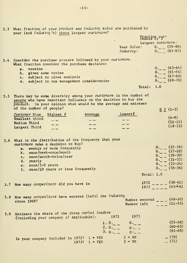
5.3 What fraction of your product and industry Bales are purchased by

your (and indue tinj 's) three largest customers?

5.

A

Fraction pucnased by 3

r-

largest customers

:

\oxiT Sales: 0. (59-60)

Industry: 0. (61-62)

Consider the purchase process followed by your oustomere.

What fraction consider the purchase decision:

a. routineb. given some review

c. subject to close analysis

d. subject to top management consideration

5.5 There may be some diversity among your auatomera in the number of

people who have important influence on the decision to buy the

product. In your opinion what would be the average and extremes

of the number of people?

Customer Size Highest // Average Lowes t^

Smallest thirdMedium ThirdLargest Third

0.

-u-

5.10 If the largest change was from .10 to .15 enter .05. Enter .05 Ifthe changes was from .15 to .10, i.e., a loss.

6.1 Selling expenses include communications, personal selling and applica-be ble overhead. If technical service is included in the selling budget

in your firm it should be included here. Reasonable judgment is neededto estimate expenses when the product is not a budget entity.

6-2 The Direct column includes everything except that included in thecolumn labeled Allowances. Allowances are those advertising andpromotional monies spent on behalf of resellers

.

6.3 Column c, Leaflets, Brochures and Catalogues, includes non-direct mailexpenses associated with these items. When sent as a mail-out includein line d. Direct mail, d, includes cost of developing the materialsas well as mailing.

-15-

5.10 Estimate the largest change in market share that any firm in this

industry experienced between 1971 and 1973: 0. (73-7^)

5.11 What fraction of your users would you say would find it

Quite Difficult: 0. (75-76)

Some Problem: 0. (77-78)

Quite Easy: 0. (79-80)

Total: 1.0

to switch to your product from a competitive one?

6. Communications. Selling. Service £ i (1-2)

6.1 What was the total amount of money (In $ thousands) spent on

selling expense for this product? 1972 ._ (4-8)

1973 . (10-14)

6.2 What was the amount of money (in $ thousands) spent on

advertising and sales promotion for this produat?Direct Allowance

1972 ._1973

6.3 Of the direct amount in 6.2, what fraction was allocated

of the following?

a. Trade & Technical Press

b. Exhibitions & Trade Shows

c. Leaflets, Brochures and Catalogues

d. Direct Mail

e. House Journal(s)

f. Press Releases

g. Televisionh. Industrial Films

i. Sales Promotion

J. Other(Describe

:

•

-16-

If your advertising/sales ratio Is .15, and industry average Is .10,then the ratio is 1.5 or 150Z — enter a '2' in (79).

See note 6.1 — judgement will be needed here also.

6.7 If your relative technical service budget is 2.5 times industryaverage(250%) enter a '1' in (23). See note 6.5.

6.8 If your expenditures would have remained the same, enter 0. If youfeel it would have been "best" (in terms of your product objectives)to have spent $100,000 more, enter 100.

6.10 If you have, say, five dedicated salesmen (1.00 of time) and five

line salesmen (.10 of each man's time), then the average salesman

spends (5 x 1.0 + 5 x .10)/10 = .55 of his time.

-17-

6.5 Compare your advertising and promotions budget (expressedas the ratio of advertising/sales) to industry averageand enter one:

1 - over 200X2 - 133-200%3 - 75-133%4 - 50-75%5 » less than 50% _ (79)

6.6 What was the total amount of money ( in $thousands) spent onpersonal selling and teahnical eerviae for this product? D 3^ (1-2)

Personal Selling Technical Service1972 ._ ._ (4-11)1973 ._ ._ (12-19)

6.7 Compare your personal selling and technical service costs(expressed as selling or service/sales) to industry average.

1 - over 200% Personal Selling _ (21)

2 = 133-200%3 - 75-133% Technical Service_ (23)

A = 50-74%5 = less than 50%

) 6.8 For this product how much more (in S thousands) would you have spent

on selling (Question 6.1) if there were no budget constraints?1972 $ ._ (25-28)

1973 $ ._ (30-33)

6.9 How many salesmen sell this product? ('35-38)

6.10 For an average salesman who sells this product, what fraction

of his time is spent on this product alone? 0. (39-40)

6.11 What fraction of an average salesman's salary comes to him as

Fixed Income 0. (42-43)

Commission 0. (44-45)

Bonus 0. (46-47)

Total: 1.0

6.12 In your most recent communications campaign about what frac-

tion of effort was allocated to the following themes:

a. Product Uniqueness

b. Awareness of Supplies

c. Product Services

d. Product Quality

e. Special Product Usesf. Inquiry Solicitation

g. Other (Specify):

0.

fl

-18-

6.13 During 1972, 1973 product plans and objectives might have beendeveloped for this product (increase market share by 10%, enternew market area, leave certain unprofitable markets, etc.). If

such plans were developed, please describe them briefly below:

How closely were the 1973 objectives met; describe what happened

in 1973 below: were they met? if not, why not, would you say?

-19-

SECTION 3:

DICTIONARY

COMPETITOR:

CUSTOMER:

INDUSTRY:

MARKET LEADER:

Normally a corporate entity with a product in the

industry.

A Buying-decision-location (User or Reseller). If

XYZ Corporation has 10 plants which independently

order the product, XYZ represents 10 customers; if

all ordering is done centrally, XYZ is a single

customer.

This should be defined to include all more or less

substitutable products or services to a given group

of customers. In some firms this is known as the

"product class." It includes the sales of your prod-

uct.

The firm in the industry with the largest market

share.

POTENTIAL CUSTOMERS : All customers using (or who would use if product were

heavily promoted) more or less substitutable products.

PRODUCT: The physical item or service that is the basis for

completing the questionnaire. Considerable flexi-

bility in the definition of product is purposely in-

cluded here: the definition should be one that has

operational meaning within the context of your organiza-

tion. The definition should never be so narrow that

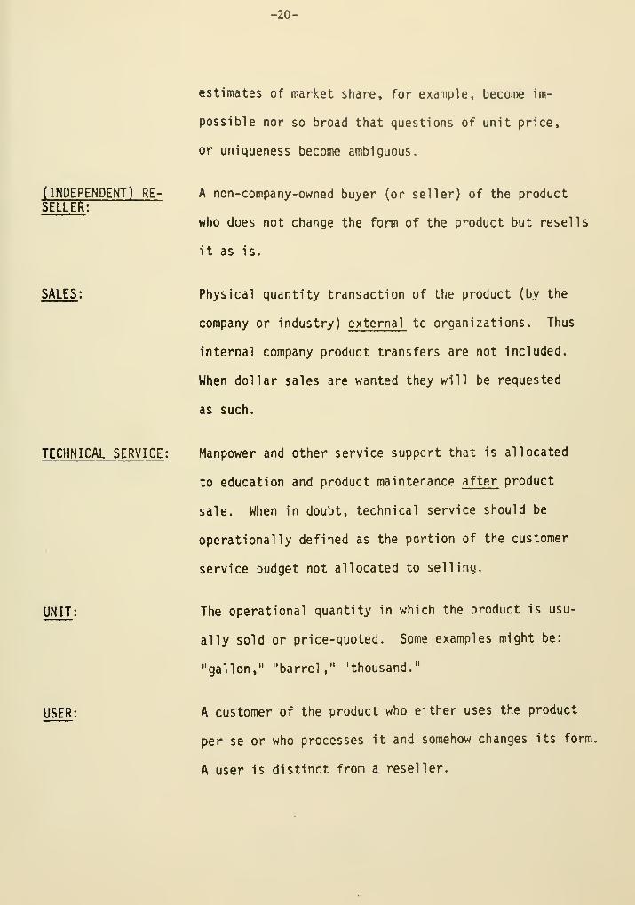
-20-

(INDEPENDENT) RE-

SELLER:

SALES:

TECHNICAL SERVICE:

UNIT:

USER:

estimates of market share, for example, become im-

possible nor so broad that questions of unit price,

or uniqueness become ambiguous.

A non-company-owned buyer (or seller) of the product

who does not change the form of the product but resells

it as is.

Physical quantity transaction of the product (by the

company or industry) external to organizations. Thus

internal company product transfers are not included.

When dollar sales are wanted they will be requested

as such.

Manpower and other service support that is allocated

to education and product maintenance after product

sale. When in doubt, technical service should be

operationally defined as the portion of the customer

service budget not allocated to selling.

The operational quantity in which the product is usu-

ally sold or price-quoted. Some examples might be:

"gallon," "barrel," "thousand."

A customer of the product who either uses the product

per se or who processes it and somehow changes its form.

A user is distinct from a reseller.

bU8 u36

B^aWJ

DEC 71984

S)EC 1 6 1985

DEC 3 1 mi

OCT 9

f£B3 1987

Y 6'®'^'

HAY 3 iai'

fJUN 2 iS90

MAR 19 1932

19136

Lib-26-67,rj/f\-^)

'!£

MAR 1 ^&

H028.M414 no.963- 77

Rhoades. Richa/A correlation of RoiD Is

73482<t D«BKS 0005486''

ii 1 11 iiiir m ii iiiiii iiii till iiii nil II iiTiTiini I iin

3 TQfiO DDL 0b6 433

HD28.M414 no.964- 77

Lorsnge, Peter /An analytical scheme to

"*'i/illlii|l!ll!lKll!jil|lll|ll|l{[|||]H

3 TDflO Q02 124 003

HD28M414 no 966- 78Reinhard. Nico/Missinq values in a rel

745179 D«BKS QOl.l?,?!"

Ilj|iii|iiiii iiiiliiiMili m3 TOfiO 0D2 112 ^62

HD28.IVI414 no.971- 78

Katz Harry Ch/Municipal labor relatio

735260 . .n.^BK? OOOS?'""

3 TQfiD DQl 10

f^S oo'

'^" -:'^\\\

525

H028.M4U no 973- 78

Lilian Gary L/The diffusion of pfiotov

73524? .O^RK^

. . .CIQ0.575Q1

3 Toao 001 100 5m

HD28.M414 no.974- 78Lilian, Gary L/AOVISOR 1 :

745181 D«BKS 0C1142?77

3 T060 002 12M 21