Advanced Physics 1/2

Theory of Magnetism

2019, terms 3/4

Harald JeschkeResearch Institute for Interdisciplinary Science, Okayama

University

Sources

This lecture is based on the books “Lecture Notes on Electron Correlation

and Magnetism” by Patrik Fazekas and “Quantum Theory of Magnetism”

by Wolfgang Nolting and Anupuru Ramakanth. In parts, it follows the

lecture notes “Theory of Magnetism” by Carsten Timm. Original papers

are used as cited in the footnotes.

1

1. Introduction

1.1 Magnetism as an effect of the electron-electron interaction

Since antiquity it was known that there is an attraction between lodestone

(magnetite, Fe3O4) and iron. Plato and Aristotle mention permanent mag-

nets. They are also mentioned in Chinese texts of the 4th century BC. Use

of a magnetic compass for navigation was first mentioned in a Chinese text

dated 1040-1044 AD but a much earlier use is possible. Apparently the

magnetic compass was first used for orientation on land, not on the sea.

Thus, magnetism at first referred to the long-range interaction between

ferromagnetic macroscopic entities. However, in this course we will focus

on the microscopic origin of the magnetic order in solids; one of these orders

is ferromagnetism.

Initially, we want to describe the effect of an external magnetic field H on

the behavior of a solid. For a weak field, the relevant response function is

the susceptibility

χ =M

H

with the magnetization density H. The probing field can be space and time

dependent. Consequently, if we introduce Fourier components of H and

M, we find in general a wave vector and frequency dependent generalized

susceptibility χ(q,ω) which fully characterizes the behavior of the systems

in weak fields. Calculating the magnetization requires solving a quantum

mechanical eigenvalue problem where the interaction of the external field

with the system is added to the microscopic Hamiltonian. The energy scale

of this interaction is µBH with the Bohr magneton

µB =

e h

2mc ≈ 9.27 · 10−21 ergG in cgs units

e h2m ≈ 9.27 · 10−24 J

T in SI units ,(1.1)

and with Gauss (G) and Tesla (T). µB is nearly equal to the spin moment

of an electron in vacuum.

2

Now how large is this energy scale µBH? In condensed matter physics,

a common energy unit is electron Volt 1 eV = 1.6 · 10−19 J, and equiva-

lent temperatures are obtained using the Boltzmann constant kB = 1.38 ·10−23 J

K = 8.6 · 10−5 eVK . This means that 1 eV corresponds to the temper-

ature 11605 K. A standard laboratory field of 5 T = 5 · 104 G then corre-

sponds to an interaction energy of µBH = 3 K. Comparing to other solid

state energy scales, this is rather small: band widths can be of the order

1 − 10 eV ∼ 104 − 105 K; Coulomb matrix elements are of similar size, and

phonons are characterized by Debye temperatures of ΘD = 100 − 1000 K.

Even spin orbit coupling is usually stronger than µBH. µBH is of the order

of the superconducting Tc of conventional superconductors; it is well known

that sufficiently strong magnetic fields can suppress superconductivity.

It would however be wrong to assume that because of the small energy

scales, no drastic change in the behavior of solids is to be expected. One

possibility is a situation of degeneracies in a system with competing energy

scales where a magnetic field can trigger strong effects. Also, if strong

correlations lead to very narrow effective bands and therefore very small

Fermi energies, as in heavy Fermion materials, laboratory fields can have

dramatic effects.

Conventionally, weak magnetism denotes the situation when the magneti-

zation of a material is induced by an external field and vanishes when the

field is turned off. Strong magnetism means that a material shows a spon-

taneous magnetization also in the absence of an external field. Formally, a

divergent static susceptibility χ(q,ω = 0) indicates the onset of magnetic

ordering.

While field induced magnetization can be attributed to a weak perturba-

tion, this is not anymore true for the origin of spontaneous magnetic or-

der. Realizable magnetic fields are rather weak, and dipole fields of atomic

moments at interatomic distances are even weaker. Let’s consider if the

magnetism of iron could be due to classical moments that align by sitting

in each others fields. In ferromagnetic iron, the moments are µat = 2.1µB,

and nearest neighbor distances are a = 2.55 A ≈ 5aB (with Bohr radius

aB = h2

me2). The fine structure constant is α = e2

hc ≈1

137 , and a Rydberg

is 1 Ry = e4m2 h2 ≈ 13.6 eV. Then the dipole-dipole interaction can be esti-

mated asµ2ata3

=(µatµB

)2( aaB

)−3α2

2 Ry ≈ 10−5 eV ≈ 0.1 K. This clearly cannot

account for a Curie temperature of 1043 K.

Spontaneous magnetic order is, in most cases, a consequence of strong

3

electron-electron interactions, rather than a secondary effect due to a weak

perturbation. The magnetism of strongly magnetic materials arises from

large terms in the Hamiltonian. Whenever band theory indicates a metal

with narrow conduction bands, magnetism arises in a natural manner (i.e.

it is one of the leading instabilities). Then the material often turns out to be

a magnetic insulator rather than a metal. Magnetic instabilities are closely

related to the problem of metal insulator transitions. Not all materials loose

their metallicity upon becoming magnetic, though: Other circumstances

like band filling play a role. There are the famous ferromagnetic metals

Fe, Co, Ni, magnetic rare earth metals Gd and Dy or the ferromagnetic

metallic oxide CrO2.

Magnetism will be discussed here in the context of electron-electron inter-

actions. Once these are strong, systems can become magnetic, they can

distort structurally, they can show metal insulator transitions, and they

might even become unconventional superconductors. The focus will here

be on the microscopic mechanisms of magnetism.

1.2 Magnetic field sources

The phenomena that can be observed experimentally are determined by

the available magnetic fields, and new field induced effects are discovered

with each progress in available magnetic field strengths. The cgs unit of

magnetic field H is Oersted, and conversion to SI is by 10Oe = 103

4πAm

. The

unit of the field B = H + 4πM is the same by value and dimension but

it is called Gauss. The SI unit is 1 Tesla = 104 G. The field of the earth is

about 0.5 G. Simple iron based permanent magnets provide a few hundred

Gauss, and powerful permanent magnets like samarium-cobalt (SmCo5) or

neodymium-iron-boron (Nd2Fe14B) have fields of 3000-4000 G. Large fields

for research are produced by electromagnets; fields of 5-30 T are routine.

There are limits to the fields that can be produced by currents through

coils because the force exerted by the field on the coil eventually exceeds

the tensile strength of the material. Resistive heating through the current

is another limiting factor. This can be avoided by the use of supercon-

ducting coils; however, superconductivity breaks down when the magnetic

field exceeds the critical field of the superconductor. Hybrid magnets with

resistive electromagnets inside a superconducting magnet can reach higher

fields, ∼ 45 T. For many experiments, it is sufficient to have an intense field

for milliseconds or microseconds; fields up to 100 T can be produced with

4

non-destructive pulsed magnets. Self-destructing pulsed magnets can pro-

duce an order of magnitude larger fields, for example very recently 1200 T

at ISSP, University of Tokyo, and constitute a very active field of research.

1.3 Some concepts at the example of magnetite

Even though magnetite was known to most ancient civilizations, it is a

complicated substance and a topic of research even today. By way of an

introduction we will learn about some of the questions that can be asked,

but not about all the answers

1.3.1 Charge states

Magnetite is an iron oxide with the formula Fe3O4; besides it, there are also

the iron oxides FeO and Fe2O3 (hematite). We can use them to analyze

the ionic bonding: We have divalent iron in Fe2+O2– and trivalent iron in

Fe3+2 O2–

3 . Now in magnetite, both divalent and trivalent iron are present:

Fe2+Fe3+2 O2–

4 . It is called a mixed valent oxide. We can try to imagine what

these charge states of iron would mean in terms of a band picture. Fe2+

and Fe3+ both have partially filled d shells, 3d5 for Fe3+ and 3d6 for Fe2+.

Now we can try to think of the resulting band as a tight binding band with

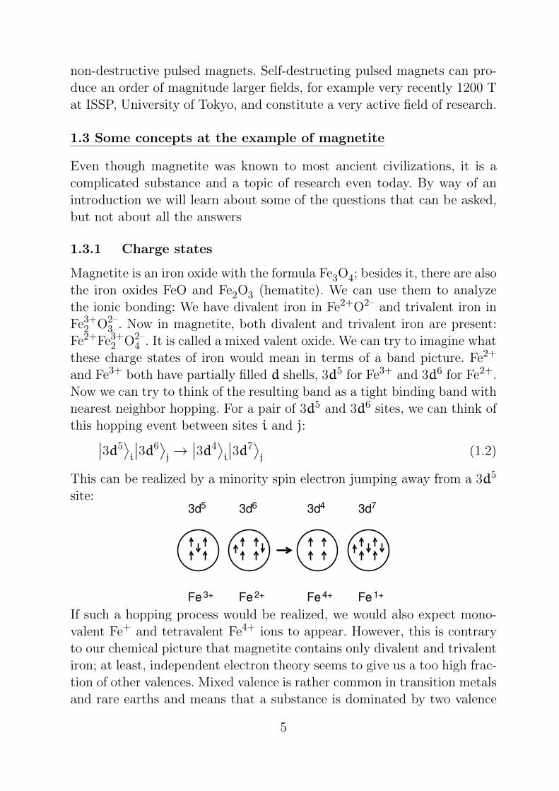
nearest neighbor hopping. For a pair of 3d5 and 3d6 sites, we can think of

this hopping event between sites i and j:∣∣3d5⟩i

∣∣3d6⟩j→∣∣3d4

⟩i

∣∣3d7⟩j

(1.2)

This can be realized by a minority spin electron jumping away from a 3d5

site:3d63d5 3d4 3d7

Fe 3+ Fe 2+ Fe 4+ Fe 1+

If such a hopping process would be realized, we would also expect mono-

valent Fe+ and tetravalent Fe4+ ions to appear. However, this is contrary

to our chemical picture that magnetite contains only divalent and trivalent

iron; at least, independent electron theory seems to give us a too high frac-

tion of other valences. Mixed valence is rather common in transition metals

and rare earths and means that a substance is dominated by two valence

5

states at the exclusion of others. Thus, in magnetite we should somehow

restrict hopping to processes that interchange Fe2+ and Fe3+:∣∣3d5⟩i

∣∣3d6⟩j→∣∣3d6

⟩i

∣∣3d5⟩j

(1.3)

Restricting hopping in this way is an example of correlated motion rather

than the usual band motion of electrons.

1.3.2 Spin states

Even equation 1.3 is still too permissive because we have not yet taken into

account the spin state. Fe2+ and Fe3+ are magnetic ions and will retain the

total spin (the magnetic moment) that they would have in free space. First

of all, we need to understand why free Fe2+ ions have total spin S = 2,

and Fe3+ ions have total spin S = 52 . Then we need to study if and how

this survives in the solid state.

So let us consider the hopping process

Fe 3+ Fe 2+ Fe 2+ Fe 3+

= 5/2S = 3/2S= 2S = 2S

This is consistent with equation 1.3 but we would consider it forbidden

because it would lead to a low spin state of Fe3+, S = 32 . Physically, the

reason to exclude such processes is the same as in the case of the valence

restriction above: It would lead from a low energy subspace to a high energy

subspace. Later, both the reason for the energetic separation of subspaces

and the way to introduce such constraints formally will be discussed.

For the special case of magnetite, it is possible to give a simple form both to

the valence constraint and to the restriction to high spin states. Magnetite

is ferrimagnetic, with an ordering temperature TN = 858 K. If we consider

temperatures of T < 200 K, we can approximate the electron motion as

hopping on the background of a frozen pattern of spin order. Magnetite has

an inverse spinel structure (Figure 1.1), AB2O4 with two crystallographi-

cally inequivalent iron sites. Below TN, spins on the two inequivalent lattice

sites are polarized in the opposite way. The tetrahedrally coordinated Asite has one Fe3+ ion, the octahedrally coordinated B site has one Fe3+

ion, one Fe2+ ion. While the opposite moment Fe3+ ions compensate each

6

Figure 1.1: In-

verse spinel struc-

ture AB2O4 of

Fe3O4: Fe3+ ions

occupy the tetrahe-

dral A sites as well

as half of the octa-

hedral B sites; the

other B sites are

occupied by Fe2+

ions.

other, a residual ferrimagnetic moment of Fe2+ on the B site remains. At

sufficiently low temperature when magnetic ordering is nearly perfect, the

only allowed hopping is that of minority spin electrons that switch Fe2+

and Fe3+ sites:

Fe 3+ Fe 2+ Fe 2+ Fe 3+

= 5/2S = 2S = 2S = 5/2S

This means that after fixing the spin order, we can forget about the spin

degree of freedom and focus only on the mobile electrons which are now

“spin free”. The problem is reduced to nearest neighbor hopping of spin-less

Fermions in a half-filled band:

Hhop = −t∑〈ij〉

(c†icj + c

†jci)

(1.4)

Here, c†i creates an electron at lattice site i, ci annihilates an electron. t is

an energy and represents the hopping amplitude.

7

1.3.3 Charge order

So far, the problem of 16 d electrons in the chemical unit cell of Fe3O4

has been reduced to a half-filled band of spin-less Fermions moving on the

the B sublattice of the inverse spinel. For a half-filled band, we would now

expect a metallic ground state. However, the resistivity of Fe3O4 shown in

Figure 1.2 clearly doesn’t show a metallic temperature dependence and is

rather high at all temperatures.

Figure 1.2: Resis-

tivity of Fe3O4 as

function of tem-

peraturea. The

temperature of the

Verwey transition

is indicated by an

arrow.

aV. V. Shchennikov,S. V. Ovsyannikov, J.Phys.: Condens. Matter 21,271001 (2009).

0.001

0.01

0.1

1

10

100

1000

10000

0 50 100 150 200 250 300 350

resis

tivity (

Ωcm

)

temperature (K)

Fe3O4

In particular, resistivity jumps up by two orders of magnitude when Fe3O4

is cooled below the so-called Verwey temperature TV ≈ 125 K. Even though

it is a transition from a semiconducting to an insulating state, it can be

considered an example of a correlation-driven metal-insulator transition.

We have accounted for substantial parts of the electron-electron repulsion

by restricting the valence states to Fe2+ and Fe3+ and by assigning defi-

nite, maximum spins to these valence states. However, an important part is

missing. In the spin-less Fermion model, the electrons are prohibited by the

Pauli principle to share the same site but there is so far nothing prevent-

ing them from sitting at nearest neighbor sites. However, the associated

Coulomb energy is large at V = e2

awith lattice spacing a. We should add

this term to the Hamiltonian:

H = Hhop +He-e = −t∑〈ij〉

(c†icj + c

†jci)+ V∑〈ij〉

ninj (1.5)

with site occupation operator ni = c†ici. This is of course a very simplified

band model but it contains some essential aspects of the Verwey transition.

8

It is an example of how model Hamiltonians are devised. The two terms

of the Hamiltonian stand for competing tendencies. For small V , the first,

kinetic energy term dominates and essentially a half-filled band with little

suppression of simultaneous occupation of neighboring sites is obtained.

On the other hand, setting t = 0 results in

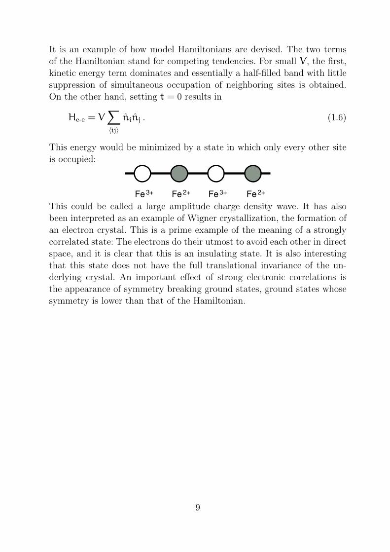
He-e = V∑〈ij〉

ninj . (1.6)

This energy would be minimized by a state in which only every other site

is occupied:

Fe 3+ Fe 2+ Fe 3+ Fe 2+

This could be called a large amplitude charge density wave. It has also

been interpreted as an example of Wigner crystallization, the formation of

an electron crystal. This is a prime example of the meaning of a strongly

correlated state: The electrons do their utmost to avoid each other in direct

space, and it is clear that this is an insulating state. It is also interesting

that this state does not have the full translational invariance of the un-

derlying crystal. An important effect of strong electronic correlations is

the appearance of symmetry breaking ground states, ground states whose

symmetry is lower than that of the Hamiltonian.

9

2. Magnetism of free atoms and ions

The study of magnetism starts with small systems – atoms, ions and

molecules – where many of the mechanisms that give rise to magnetic

ordering are already active as soon as there are two interacting electrons.

The tendency to form a high spin ground state in a small system is related

to a ferromagnetic state in a solid, the tendency to align antiparallel and

form a spin singlet is related to antiferromagnetism. On the other hand,

when electrons are essentially localized to ions, the properties of the iso-

lated ions are directly relevant also for the solid, as is the case for rare

earth ions.

2.1 Hartree approximation for the electron shell

We cannot exactly solve the many-body problem of a nucleus with many

electrons. In the simplest non-trivial approximation, the Hartree approx-

imation, a given electron moves in a potential resulting from the nucleus

and the average density of the other electrons; it is important that the self-

interaction, the interaction of the electron with its own averaged charge

density is excluded. The total potential is

Veff(r) = −

1

4πε0

Ze2

r−

1

4πε0

∫d3r ′

eρr(r ′)

|r−

r ′|

(2.1)

where Z is the atomic number of the nucleus, the electron charge is −e < 0,

and ρr(r ′) < 0 is the charge density at

r ′ of the other electrons if the given

electron is atr. Veff(

r) is spherically symmetric due to the isotropy of

space, but ρr(r ′) as a function of

r ′ is not spherically symmetric except

forr = 0. For the electron at

r we solve the single-particle Schrodinger

equation( p2

2m+ Veff(

r))ψ(

r) = Eψ(

r) (2.2)

10

From a separation of variables and using the spherical symmetry, the eigen-

functions are

ψnlm(r) = Rnl(r)Ylm(ϑ,φ) (2.3)

with principal quantum number n = 1, 2, 3, . . . , orbital angular momentum

quantum number l = 0, 1, 2, . . . ,n−1 and magnetic quantum numberm =−l,−l+1, ..., l. The angular part is the same for any spherically symmetric

potential and is given by the spherical harmonics Ylm(ϑ,φ). Eigenenergies

εn,l only depend on n, l in the present approximation. Including a factor

of 2 from spin s = 1/2, the εn,l are 2(2l+ 1)-fold degenerate. Completely

full shells comprising all orbitals with a given quantum number n, l have

〈∑

i

li〉 = 0 and 〈∑isi〉 = 0, i.e. vanishing total angular moment because

for every electron there is another one with opposite 〈

li〉, 〈si〉. The total

magnetic moment of filled shells also vanishes. Therefore, magnetic ions

require incompletely filled shells.

In the ground states, we need to fill the Hartree orbitals starting from the

lowest in energy. For a shell containing p electrons (with p < 2(2l + 1)),the number of possibilities of doing this is given by(

2(2l+ 1)p

).

This represents the degeneracy of the many-particle state. For a filled state,

we get no degeneracy: (2(2l+ 1)2(2l+ 1)

)= 1 .

2.2 Beyond the Hartree approximation

The large degeneracy we found is partially lifted by the Coulomb repulsion

beyond the Hartree approximation. The Coulomb interaction

VC =1

4πε0

1

2

∑i 6=j

e2

|ri −

rj|

(2.4)

commutes with the total orbital angular momentum of the shell

L =∑i

lias VC is spherically symmetric, and with the total spin of the shell

S =∑isi as well because the Hamiltonian doesn’t depend on it:

[

S,H]− = 0 , [

L,H]− = 0 (2.5)

11

The Hamiltonian also commutes with

L2 and with

S2. Furthermore, the

total angular momentum of the shell

J =

L+

S (2.6)

commutes with the Hamiltonian

[

J,H]− = 0 . (2.7)

Physically, this means that

L =

p∑i=1

m(i)l , S =

p∑i=1

m(i)s , J (2.8)

are good quantum numbers;m(i)l andm

(i)s are the magnetic quantum num-

bers of the electrons. We can also say that there exists a simultaneous set

of eigenstates for the operators

H, J2, Jz,L2,Lz,S

2,Sz ,

and states can be labeled by the corresponding quantum numbers

| . . . 〉 = |J,MJ,L,ML,S,MS〉 (2.9)

Here, S is the maximum possible value of 〈Sz〉, L is the maximum possible

value of 〈Lz〉. For example,

J2| . . . 〉 = h2J(J+ 1)| . . . 〉 Jz| . . . 〉 = hMJ| . . . 〉J = |L− S|, . . . ,L+ S − J 6MJ 6 +J (2.10)

The other angular momentum operators act in similar fashion. The energy

eigenvalues of the Hamiltonian

H| . . . 〉 = E(0)JLS| . . . 〉 (2.11)

will depend on J, L, S, but in the absence of a magnetic field, they will be

degenerate with respect to MJ, ML and MS.

If we apply the raising operator L+ = Lx + iLy to |ψ〉 and obtain a |ψ ′〉with M ′

L = ML + 1, we reach a new state that has the same energy as

the old one because [H,L+] = 0. There are (2L + 1)(2S + 1) states that

are connected by L± and by S± (S− = Sx − iSy, S+ = Sx + iSy); the(

2(2l+ 1)p

)-fold degenerate states split into multiplets with fixed S and

L and degeneracies (2L + 1)(2S + 1). Typically, energy splitting between

multiplets are much larger than 1 eV so that for magnetic problems, we

only need to know the ground state multiplet.

12

2.2.1 Hund’s rules for LS coupling

We assume here that the Coulomb interaction HC is significantly larger

than the spin-orbit coupling HSO

HC HSO

which leads us to the Russell-Saunders- or LS-coupling. This is relevant for

light nuclei.

The empirical Hund’s rules tell us how to build the ground-state LS mul-

tiplet for given L and S, and for p electrons filled into a shell with orbital

angular momentum quantum number l:

1st Hund’s rule: The ground state multiplet has the largest possible S.

(The maximum S corresponds to the largest possible value of 〈Sz〉).

S =1

2

[(2l+ 1) − |2l+ 1 − p|

]2nd Hund’s rule: If the 1st Hund’s rule leaves several possibilities, the

state with maximum L is lowest in energy:

L = S|2l+ 1 − p|

(The maximum L corresponds to the largest possible value of 〈Lz〉).

A short qualitative explanation for the 1st Hund’s rule is that the same spin

together with the Pauli principle means that the electrons are on average

further apart, reducing the Coulomb repulsion. Also the aligned orbital

momenta, i.e. rotation in the same sense, of the second rule optimizes

distance between electrons and reduces Coulomb energy.

The multiplets are labeled as 2S+1L where a letter is used for L:

L = 0 1 2 3 4 5 6 . . .

X = S P D F G H I continuing alphabetically

We can count the number of distinct states within the LS multiplets as

L+S∑J=|L−S|

(2J+ 1) = (2S+ 1)(2L+ 1) (2.12)

Often (not always), these states are ordered according to the

13

Table 2.1: Atomic term scheme for an f shell occupied by p electrons. ↑represents spin projection 1/2, ↓ represents spin projection −1/2.

p ml

3 2 1 0 -1 -2 -3 S L J term

1 ↑ 1/2 3 5/2 2F5/2

2 ↑ ↑ 1 5 4 3H4

3 ↑ ↑ ↑ 3/2 6 9/2 4I9/24 ↑ ↑ ↑ ↑ 2 6 4 5I4

5 ↑ ↑ ↑ ↑ ↑ 5/2 5 5/2 6H5/2

6 ↑ ↑ ↑ ↑ ↑ ↑ 3 3 0 7F0

7 ↑ ↑ ↑ ↑ ↑ ↑ ↑ 7/2 0 7/2 8S7/2

8 ↑↓ ↑ ↑ ↑ ↑ ↑ ↑ 3 3 6 7F6

9 ↑↓ ↑↓ ↑ ↑ ↑ ↑ ↑ 5/2 5 15/2 6H15/2

10 ↑↓ ↑↓ ↑↓ ↑ ↑ ↑ ↑ 2 6 8 5I8

11 ↑↓ ↑↓ ↑↓ ↑↓ ↑ ↑ ↑ 3/2 6 15/2 4I15/212 ↑↓ ↑↓ ↑↓ ↑↓ ↑↓ ↑ ↑ 1 5 6 3H6

13 ↑↓ ↑↓ ↑↓ ↑↓ ↑↓ ↑↓ ↑ 1/2 3 7/2 2F7/2

14 ↑↓ ↑↓ ↑↓ ↑↓ ↑↓ ↑↓ ↑↓ 0 0 0 1S0

3rd Hund’s rule: For the total angular momentum of the shell,

J = |

L−

S| in case the shell is less than half filled (p 6 (2l+ 1)),

J =

L+

S in case the shell is more than half filled (p > (2l+ 1)),

which means

J = S|2l− p| .

Table 2.1 gives the terms for an f shell (e.g. 4f, relevant for rare earths),

occupied by p electrons.

2.3 Spin-orbit coupling

Experimentally, the magnetic moment of an electron is

ms = −gµB

s h

with g ≈ 2.0023. This cannot be explained with a classical calculation.

A classical estimate of g based on the assumption that an electron is a

spinning charged sphere with angular momentums would only lead to

14

g = 1. However, relativistic Dirac quantum theory gives g = 2, and the

remaining≈ 0.0023 are due to small corrections arising from the interaction

of the electronic charge with the electromagnetic field it generates; this can

be calculated precisely with quantum electrodynamics.

We will see now that also for the many-particle states of ions, a relativistic

description is necessary. The starting point for the derivation is the non-

relativistic v c limit of the Dirac equation which gives rise to the two-

component Pauli theory. However, we have to go further in perturbation

theory, including terms of the order v2

c2. This higher order approximation

is done formally correctly using the Foldy-Wouthuysen transformation. A

static electric potential φ of the nucleus is considered. One obtains the

following Hamiltonian in spinor space:

H =p2

2m+ φ(

r) −

p4

8m3ec

2+

h2

2m2ec

2

1

r

∂φ

∂r

s ·

l+ h2

8m2ec

2∇2φ (2.13)

Here, the first two terms are the non-relativistic H0, the third term is a

relativistic correction to the kinetic energy, the fourth term contains the

spin-orbit coupling HSO, and the last term is a correction to the potential,

known as the Darwin term.

We will now consider the spin-orbit coupling term for the central potential

of the nucleus

HSO = − h2

2m2ec

2

Ze2

4πε0

1

r

∂

∂r

1

r

s ·

l = h2

2m2ec

2

Ze2

4πε0

s ·

l

r3=µ0

4πgµ2

BZ

s ·

l

r3,

where we assume g = 2 and use µB = e h2me

and c = 1µ0ε0

.

The operator of spin-orbit coupling for several electrons in an incompletely

filled shell is then

HSO =µ0

4πgµ2

BZ∑i

si ·

li

r3i. (2.14)

In principle, not only the bare nuclear potential but the full effective poten-

tial of the Hartree approximation should be taken into account; however,

this is done in practice by replacing the atomic number Z by an effective

Zeff < Z. Next, we treat HSO as a weak perturbation to H0 and evaluate

the contribution of the spin-orbit coupling to the energy:

ESO :=⟨HSO

⟩=µ0

4πgµ2

BZ∑i

⟨si ·

li

r3i

⟩. (2.15)

15

For free ions, the radial wave function Rnl for all orbitals of the nl shell is

the same; therefore

ESO =µ0

4πgµ2

BZ∑i

⟨1

r3

⟩nl

⟨si ·

li⟩

. (2.16)

Now we call electrons with spin parallel to

S spin up (↑) and the others

spin down (↓). Also, thesi and

li commute. Thus

ESO =µ0

4πgµ2

BZ∑i

⟨1

r3

⟩nl

( ∑i

spin up

⟨

S ·

li

2S

⟩−∑i

spin up

⟨

S ·

li

2S

⟩).

We distinguish three cases:

(i) If the shell is less than half filled (nnl < 2l+ 1), all spins are aligned

and the spin down sum doesn’t contain any terms:

ESO =µ0

4πgµ2

BZ

⟨1

r3

⟩nl

1

2S

⟨S·∑i

li⟩=µ0

4πgµ2

BZ

⟨1

r3

⟩nl

1

2S

⟨S·

L⟩=: λ

⟨S·

L⟩

(2.17)

with

λ =µ0

4πgµ2

BZ

⟨1

r3

⟩nl

1

2S.

(ii) If the shell is more than half filled (nnl > 2l + 1), the spin up sum

vanishes because it contains

l∑ml=−l

〈lml|

l|lml〉 = 0

and we obtain

ESO = −µ0

4πgµ2

BZ

⟨1

r3

⟩nl

1

2S

⟨S ·

L⟩=: λ

⟨S ·

L⟩

(2.18)

with

λ = −µ0

4πgµ2

BZ

⟨1

r3

⟩nl

1

2S.

(iii) If the shell is half filled (nnl = 2l + 1), both spin up and spin down

sums vanish and we get ESO = 0. Note that at higher orders in

perturbation theory, there is a nonzero contribution.

16

In summary, the spin-orbit coupling in a free ion behaves, within pertur-

bation theory, like a term HSO = λ⟨S ·

L⟩

in the Hamiltonian, with λ > 0

for less than half filled shells and λ < 0 for more than half filled shells.

As a consequence of spin-orbit coupling HSO, even in the absence of an

external magnetic field (

B0 = 0)

l ands do not commute with the Hamil-

tonian.

One can show that[l · s,

l]−= i h

(l×

s)= −

[l · s,

s]−

.

On the other hand, [l · s,

j]−= 0 with

j =

l+s .

Furthermore, [l · s,

j2]−=[l · s,

l2]−=[l · s,

s2]−= 0 .

This means that the energy eigenstates can be classified by j, mj, l and s(which are good quantum numbers) but not by ml and ms. HSO couples,

i.e. hybridizes the states with different ml and ms.

HSO partially lifts the degeneracy of the LS-multiplet (here the doublet as

our treatment is for one electron, j = l± 1/2). Due to

j =

l+sy 2

(l · s)=

j2 −

l2 −s2

HSO produces a fine structure of the energy terms

E(0)nlj = E

(0)nl + λnl h

2[j(j+ 1) − l(l+ 1) − s(s+ 1)] (2.19)

with energy E(0)nlj in the absence of spin-orbit coupling. The constant λnl is

λnl = −e

2m2ec

2

⟨nls∣∣∣1r

dφ

dr

∣∣∣nls⟩ .

Thus, terms with j = l ± 1/2 have different energies for l 6= 0 while the

2j+ 1-fold degeneracy due to mj remains.

2.4 Magnetic moments of ions

A problem arises when we want to calculate the magnetic moment of an

ion with quantum number S, L, J: Using g = 2 for the g factor of the

electron, the magnetic moment ismJ =

mS +

mL = −2µB

S− µB

L = −µB

((2

S+

L)= −µB

(J+

S)

17

ButmJ does not commute with the Hamiltonian because of the spin-orbit

coupling term λ

L ·

S (

J does commute but

S does not). Therefore,

J is a

constant of motion butmJ is not; we can think of

S and

L and thusmJ as

rotating around the fixed vector

J (see Figure 2.1).

Figure 2.1: Nei-

ther

L,

S normJ

are constants of

motion, only

J.

S

S

LJ

J+S

Jm

The typical time scale of this rotation should be h|λ|

. For “slow” experi-

ments like magnetization measurements, only a time averagedmobs will

be observable. We can determine it by projectingmJ on the direction of

the constant

J:

mobs =

(mJ ·

J)J

J ·

J= −µB

[(J+

S)·

J]J

J ·

J= −µB

J− µB

(S ·

J)J

J ·

J

= −µB

J+µB

2

(J−

S)2

−

J ·

J−

S ·

S

J ·

J

J and with

J−

S =

L

mobs = −µB

J−µB

2

J(J+ 1) + S(S+ 1) − L(L+ 1)

J(J+ 1)

J =: −gJµB

J (2.20)

after introducing the Lande g factor

gJ = 1 +J(J+ 1) + S(S+ 1) − L(L+ 1)

2J(J+ 1)(2.21)

gJ satisfies 0 6 gJ 6 2 and can be smaller than the orbital value gL = 1.

18

3. Diamagnetism

Diamagnetism is defined by χdia < 0 where χdia = constant. The simple

explanation is that this is an induction effect: The external field induces

magnetic dipoles which, according to Lenz’s law, are oriented antiparallel

to the field and therefore χ is negative. We will see in a moment that

strictly speaking, this easily understandable picture is not quite true, as

without quantum mechanical effects, there is not even diamagnetism.

Empirically, the effect of diamagnetism is displayed by all materials; how-

ever, they are only called diamagnets if no other, stronger type of mag-

netism like paramagnetism or collective magnetism is present. Examples

for diamagnets are almost all organic substances, metals like Bi, Zn and

Hg, nonmetals like S, I and Si, and superconductors for T < Tc; in fact they

are perfect diamagnets: χdia = −1 which is called the Meissner-Ochsenfeld

effect.

3.1 Bohr-van-Leeuwen theorem

The Bohr-van Leeuwen theorem states: Magnetism is a quantum mechani-

cal effect. Strictly classically, there cannot be either dia-, para- or collective

magnetism.

Proof: We assume a solid of identical ions with translational symmetry.

Then the magnetization is

M =N

V〈 m〉 ,

wherem is the magnetic moment of the individual ion, andN is the number

of ions in volume V . The magnetic moment can be related to the energy

W of the magnetic system and to the Hamiltonian H:

m = −

∂W

∂

B0

= −∂H

∂

B0

, (3.1)

where H is the classical Hamiltonian function of a single ion. The classical

19

average can be calculated by

〈 m〉 = 1

Z∗

∫· · ·∫dx1 . . .dx3Ne

∫dp1 . . .dp3Ne

me−βH (3.2)

with the number of electrons Ne and with the classical partition function

Z =Z∗

Ne!h3Ne

given by

Z∗ =

∫· · ·∫dx1 . . .dx3Ne

∫dp1 . . .dp3Nee

−βH (3.3)

with the inverse temperature β = 1kBT

. Then

1

βZ

∂Z

∂

B0

=1

βZ∗∂Z∗

∂

B0

=1

βZ∗

∫· · ·∫dx1 . . .dx3Ne

∫dp1 . . .dp3Nee

−βH

(− β

∂H

∂

B0

)=

1

Z∗

∫· · ·∫dx1 . . .dx3Ne

∫dp1 . . .dp3Nee

−βH m = 〈 m〉

(3.4)

Thus,

〈 m〉 = 1

βZ

∂Z

∂

B0

. (3.5)

If we can show that Z doesn’t change when an external field

B0 is switched

on, the theorem is proven. The general form of H in the presence of a

magnetic field

B0 = ∇×

A is

H =1

2m

Ne∑i=1

(pi + e

Ai)2 +H1(x1, . . . , x3Ne) (3.6)

where H1 represents the electron-electron interactions. Then we can write

for the partition function

Z∗ =

∫. . .

∫dx1 . . .dx3Nee

−βH1(x1, . . . , x3Ne)×

×∫∞−∞· · ·

∫∞−∞ dp1 . . .dp3Nee

−β

2m

Ne∑i=1

(pi + e

Ai)2

(3.7)

20

As the momentum integration runs from −∞ to ∞, we can substituteui =

pi + e

Ai without changing the limits of integration:

Z∗ =

∫. . .

∫dx1 . . .dx3Nee

−βH1(x1, . . . , x3Ne)×

×∫∞−∞· · ·

∫∞−∞ dp1 . . .dp3Nee

−β

2m

Ne∑i=1

u2i

(3.8)

which obviously is independent of the magnetic field, Z 6= Z(B0). Thus,

the average magnetic moment vanishes in all cases:

〈 m〉 ≡ 0 .

Rigorously, classically, there is no magnetism, and it is best to always argue

quantum mechanically.

In matter, we have charged particles in motion which respond to an ex-

ternal magnetic field

B0. Either the system contains permanent magnetic

moments. Then they will order in a field and give rise to collective phe-

nomena like paramagnetism, ferromagnetism, antiferromagnetism or fer-

rimagnetism. Or, the field itself induces the magnetic moments. This is

called diamagnetism and is only observable if no permanent moments are

present. We can distinguish between the diamagnetism of insulators which

is called Larmor diamagnetism and diamagnetism of itinerant electrons in

metals which is called Landau diamagnetism.

3.2 Larmor diamagnetism

As diamagnetism is only observable in a system without other kinds of

magnetism, we consider a solid made up out of ions with completely filled

shells. For the ground state, we have

J|0〉 =

L|0〉 =

S|0〉 = 0 (3.9)

We switch on an external magnetic field given by

B0 = µ0

H = (0, 0,B0)

and look for the response of the system, i.e. the field induced magnetic

moment, the magnetization. We consider an insulator where all electrons

are strictly localized. Then

M(B0) =N

V〈0| m|0〉 (3.10)

21

for N ions in volume V . We already know that magnetic energies ≈ µBB0

are usually so small that the system remains in the ground state |0〉 in

the average. We now need the Hamiltonian in a homogeneous magnetic

field from which we obtain the magnetization asm = −

∂H

∂

B0

. We consider

only the electrons and ignore the interactions between them and with the

nucleus for the time being. We choose the vector potential in the Coulomb

gauge so that

B0 = ∇×

A with ∇ ·

A = 0 . (3.11)

This can be achieved by

A =1

2

B0 ×r .

The kinetic energy without field is

T0 =

n∑i=1

p2i

2

for n electrons with charge −e so that e > 0. In the field, the canonical

momentumpi is different from the mechanical momentum m

vi:

pi = m

vi − e

A(ri) . (3.12)

Then we have for the kinetic energy

T =1

2m

n∑i=1

(pi+e

A(ri))2

=1

2m

n∑i=1

[p2i+e

(pi·

A(ri)+

A(ri)·

pi)+e2

A2(ri)]

(3.13)

In general, operatorspi and

A(ri) do not commute, but in Coulomb gauge

they do:pi ·

A(ri) =

h

i

(∇i ·

A︸ ︷︷ ︸=0

+

A · ∇i)=

A(ri) ·

pi .

Therefore, the kinetic energy becomes

T = T0 +e

m

n∑i=1

A(ri) ·

pi +

e2

2m

n∑i=1

A2(ri) (3.14)

With the field

B0 in z direction

B0 = (0, 0,B0), the vector potential is

A =1

2

B0 ×r =

B0

2(−y, x, 0) . (3.15)

22

The scalar product

A(ri) ·

pi can be expressed by the orbital angular

momentum

li of electron i:

A(ri) ·

pi =

B0

2(−yipix + xipiy) =

1

2B0liz =

1

2

B0 ·

li .

Then using the total orbital angular momentum

L =∑ni=1

li, we have

T = T0 +µB

h

L ·

B0 +e2B2

0

8m

n∑i=1

(x2i + y

2i

). (3.16)

In this derivation we have neglected the spin

S of the electrons; we already

know that the field couples not only to

L but actually to

J =

L+2

S. Thus,

two terms in the Hamiltonian contain the magnetic field,

HZ = −µB h(Lz + 2Sz)B0 and Hdia =

e2B20

8m

n∑i=1

(x2i + y

2i

)(3.17)

Performing the average for the first term (considering completely filled

shells, Equation 3.9) gives ⟨0

∣∣∣∣∂HZ

∂

B0

∣∣∣∣0⟩ = 0 .

We are left with

M(B0) = −N

V

⟨0

∣∣∣∣∂Hdia

∂

B0

∣∣∣∣0⟩ (3.18)

Due to the spherical symmetry of the ion (noble gas configuration), we

have

n∑i=1

〈0|x2i |0〉 =

n∑i=1

〈0|y2i |0〉 =

n∑i=1

〈0|z2i |0〉 =

1

3

n∑i=1

〈0|r2i |0〉 .

As x and y components of the magnetization vanish, we find for the zcomponent

M(B0) = −Ne2

6mVB0

n∑i=1

〈r2i 〉 . (3.19)

23

The diamagnetic susceptibility is obtained by differentiating again with

respect to B0:

χdia = µ0

(∂M

∂

B0

)T

= −Ne2

6mV

n∑i=1

〈0|r2i |0〉 , (3.20)

where the negative sign indicates diamagnetism. The external field induces

a moment whose field is directed opposite to the applied field.

To estimate the order of magnitude of χdia, we first note that in the liter-

ature, usually the molar susceptibility is given:

χdiam =

NAV

Nχdia

[cm3

mol

](3.21)

with Avogadro number NA = 6.022 · 1023 mol−1. The average ion radius

〈r2〉 = 1

n

n∑i=1

〈0|r2i |0〉

can be expressed in units of the Bohr radius

aB =4πε0 h

2

me2= 0.529 A .

Then the molar susceptibility is

χdiam = −0.995 · 10−5n

⟨r2

a2B

⟩ [cm3

mol

], (3.22)

where⟨r2

a2B

⟩is of the order of 1. Thus, χdia

m is very small and diamagnetism

is only observable when it is not shadowed by paramagnetism or collective

magnetism.

Table 3.1: Examples of diamagnetic molar susceptibilities χdiam in

10−6cm3/mol.

He -1.9 Li+ -0.7

F− -9.4 Ne -7.2 Na+ -6.1

Cl− -24.2 Ar -19.4 K+ -14.6

Br− -34.5 Kr -28.0 Rb+ -22.0

I− -50.6 Xe -43.0 Cs+ -35.1

24

Examples are noble gases and simple ionic crystals like alkali metal halides

for which contributions of cations and anions add up.

In Table3.1, the electron number increases within each column, and so

does |χdiam | (see Eq. 3.22). In each row, electron number is the same but the

nuclear charge Z increases, increasing the attractive force on the electron

shells and thus shrinking the size of the ion 〈r2〉 from left to right; thus,

|χdiam | decreases.

3.3 Landau diamagnetism

There is also a diamagnetic contribution to the susceptibility due to (nearly)

free electrons in metals; free electrons in an electron gas lead to charge cur-

rents in a magnetic field which generate magnetic moments. This would

still be true if the electrons had no spin (no spin magnetic moment). This

diamagnetic response, due to the Bohr-van Leeuwen theorem, has to be a

quantum-mechanical phenomenon.

3.3.1 Two-dimensional electron gas

As a first step, we consider a two-dimensional electron gas in a uniform

magnetic field based on the single-electron Hamiltonian

H =1

2m

[p+ e

A(r)]2

(3.23)

with charge −e. The Zeeman term which would lead to paramagnetism is

neglected here. Without loss of generality, we assume the uniform field to

point in z direction,

B0 = (0, 0,B0). We choose the so-called Landau gauge

A(r) = (−B0y, 0, 0)

which gives

B0 = ∇×

A =

∂y0 − ∂z0−∂zB0y− ∂x0∂x0 + ∂yB0y

=

0

0

B0

. (3.24)

Thus

H =1

2m(px − eB0y)

2 +1

2mp2y (3.25)

we have [H,px] = 0 as H doesn’t contain x; px is a constant of motion,

and we can replace it by its eigenvalue hkx. If we define y0 := heB0kx and

25

ωc :=eB0m

with cyclotron frequency ωc, we obtain

H =1

2mp2y +

m

2ω2

c(y− y0)2 . (3.26)

This Hamiltonian describes a harmonic oscillator with potential minimum

shifted to y0. It has the eigenvalues

En,kx = hωc

(n+

1

2

), n = 0, 1, 2, . . . (3.27)

This is a huge degeneracy because the energies do not depend on kx. The

apparent asymmetry between x and y direction in H is gauge dependent

and therefore without physical consequence. We could have chosen the

vector potential to point in any direction within the xy plane. The isotropy

of the two-dimensional space is not broken by the choices of a special gauge.

The magnetic field transforms the spectrum of the two-dimensional electron

gas

Ek=

h2

2m

(k2x + k

2y

)into a discrete spectrum of Landau levels enumerated by n. For B0 = 0,

the density of states is

D(ε) =

∫d2k

(2π)2δ

(ε−

h2k2

2m

)=

1

2π

∫∞0dkkδ

(ε−

h2k2

2m

)=︸︷︷︸

u=k2,du=2kdk

1

4π

∫∞0duδ

(ε−

h2u

2m

)=

1

4π

∫∞0dE

2m h2δ(ε− E)

=m

2π h2for ε > 0

(3.28)

Thus, the density of states is constant. For B0 > 0, it is replaced by δfunction peaks (Figure 3.1).

We can now determine the degeneracy of the Landau levels. Since the total

number of states does not change, the Landau levels must accommodate

these states; thus, the degeneracy of the first one, and all others, is (for an

electron gas enclosed in a sample with area L2)

NL = L2

∫ hωc

0dεD(ε) =

m

2π h2 hωcL

2 =m

2π h

eB0

mL2 =

eB0

hL2 (3.29)

26

h/2ωc 3h/2ωc 5h/2ωc 7h/2ωc

D(ε)

ε

firs

t Landau level

second L

andau level

Figure 3.1: Den-

sity of states of

two-dimensional

electron gas at fi-

nite magnetic field

B0 > 0.

At low temperature, the low energy states are filled successively until all

N electrons are accommodated. If

N = 2nNL with n = 1, 2, . . .

the n lowest Landau levels are completely filled and the others are empty.

The factor 2 is due to the two spin directions. In case that N2NL

is not an

integer, the highest Landau level is partially filled. Landau level quantiza-

tion is one of the key ingredients of the integer quantum Hall effect. For

calculating the total energy of N electrons, we define bxc as the largest

integer smaller or equal to x, and n =⌊N

2NL

⌋; then

E =

n−1∑n=0

2NL hωc

(n+

1

2

)+ (N− n2NL) hωc

(n +

1

2

). (3.30)

The first term describes the filled Landau levels, and the second the par-

tially filled one. With the filling factor ν := N2NL

, the energy per electron

is

E

N=

n−1∑n=0

2

ν hωc

(n+

1

2

)+(

1 −2n

ν

) hωc

(n +

1

2

). (3.31)

with n =⌊ν2

⌋. This function is continuous but not everywhere differentiable

(see Figure 3.2). Bt is the field for which ν = 2, i.e. for which the lowest

Landau level is completely filled:

N

NL=

Nh

eBtL2

!= 2 y Bt =

hN

2eL2

27

Figure 3.2: En-

ergy of the two-

dimensional elec-

tron gas as func-

tion of magnetic

field B0. Bt/3 Bt/2 Bt

E (

arb

. units)

B0

The areal magnetization

M = −1

L2

∂E

∂B0

shows oscillations that are periodic in 1B0

. These are the de Haas-van Alphen

oscillations (see Figure 3.3).

Figure 3.3: Mag-

netization of the

two-dimensional

electron gas as

function of mag-

netic field B0.−0.5

0

0.5

Bt/3 Bt/2 Bt

M (

arb

. u

nits)

B0

The limit limB0→0M does not exist; neither does the limit limB0→0 χ for

the susceptibility χ = ∂M∂B0

. This unphysical result is due to the assumption

of zero temperature T = 0. At any T > 0, the thermal energy kBT will be

large compared to the energy spacing hωc between the Landau levels for

sufficiently small B0. In this regime, the discreteness of the Landau levels

28

can be neglected, and the energy becomes

EN2NL

∼=

∫ N2NL

0dn 2NL hωcn =

2eB0

hL2

heB0

m

[n2

2

] Nh

2eB0L2

0

=e2B2

0

πmL21

2

N2h2

4e2B20L

4=N2h2

8πm

1

L2. (3.32)

Thus, the areal magnetization vanishes:

M = −1

L2

∂E

∂B0= 0

We could have guessed this result: Smearing out the rapid oscillations at

small B0 would lead to M = 0. Thus, χ = ∂M∂B0

= 0 in this limit; the

diamagnetic susceptibility of the two-dimensional electron gas vanishes.

3.3.2 The three-dimensional electron gas

The Hamiltonian of free electrons in three dimensions in the presence of a

uniform magnetic field

B0 = B0ez is

H =1

2m

[p+ e

A(r)]2

=1

2mp2y +

m

2ω2

c(y− y0)2 +

1

2mp2z , (3.33)

using again the Landau gauge A = (−B0y, 0, 0). Now we obtain free mo-

tion in z direction in addition to shifted harmonic oscillators in the xyplane. The eigenenergies are

En,

k= hωc

(n+

1

2

)+

h2k2z

2m, n = 0, 1, 2, . . . (3.34)

The density of states is thus a sum of the densities of states of the one-

dimensional electron gas, shifted to the minimum energies hωc

(n + 1

2

),

n = 0, 1, 2, . . . . The resulting density of states is for one spin direction

D(ε) =NL

L2

∞∑n=0

1

π h

√√√√ m

2(ε− hωc

(n+ 1

2

))Θ(ε− hωc

(n+

1

2

))

=1

π h

√m

2

NL

L2

∞∑n=0

Θ

(ε− hωc

(n+ 1

2

))√ε− hωc

(n+ 1

2

) (3.35)

29

Figure 3.4: Den-

sity of states of

three-dimensional

electron gas at fi-

nite magnetic field

B0 > 0. h/2ωc 3h/2ωc 5h/2ωc 7h/2ωc

D(ε)

ε

For kBT hωc, the low-energy states are filled up until all electrons

are accommodated, as in the case of the two-dimensional electron gas.

As before, we expect special features whenever the chemical potential µreaches hωc

(1 + 1

2) with n = 1, 2, . . . . Since µ is roughly constant in

three dimensions (it has a saw-tooth behavior in two dimensions, with

discontinuities at Bt,Bt/2,Bt/3, . . . ) while hωc ∝ B0, the total energy

E(B0) and therefore the magnetization M = − 1V∂E∂B0

(with volume V) will

have features which are periodic in 1B0

; these are again de Haas-van Alphen

oscillations. They become visible in large magnetic fields.

In the context of conduction electron diamagnetism, we are interested in

the susceptibility for small fields. We have hωc kBT , and for a typical

metal, we assume kBT µ. It is useful to define the iterated integrals of

the density of states

P1(x) :=

∫ x0dεD(ε) ,

P2(x) :=

∫ x0dεP1(ε) , (3.36)

The total number of electrons is

N = 2VP1(µ)

where the factor 2 accounts for two spin directions. The total energy is

E = 2V

∫µ0dε εD(ε) .

30

Partial integration gives

E = 2V

[µP1(µ) −

∫µ0dεP1(ε)

]= µN− 2VP2(µ) . (3.37)

The explicit expression for P2(µ) is

P2(µ) =1

π h

√m

2

NL

L2

∞∑n=0

4

3

(µ− hωc

(n+

1

2

))32

Θ

(µ− hωc

(n+

1

2

)).

(3.38)

Since hωc µ, we can replace the sum over n by a integral. The Poisson

summation formula provides the correct expression for this:

∞∑n=0

f(n+

1

2

)=

∫∞0dx f(x) + 2

∞∑s=0

(−1)s∫∞

0dx f(x) cos(2πsx) (3.39)

We find

P2(µ) =1

π h

√m

2

NL

L2

4

3

∫ µ hωc

−12

0dx (µ− x hωc)

32

+ 2

∞∑s=1

(−1)s∫ µ

hωc−1

2

0dx (µ− x hωc)

32 cos(2πsx)

=

1

π h

√m

2

NL

L2

4

3

2

5

µ52

hωc−

1

10√

2( hωc)

32 + 2

∞∑s=1

(−1)s3

8π2

hωc√µ

s2

+ oscillating terms

(3.40)

The oscillating terms contain cos(

2πsµ hωc

)or sin

(2πsµ hωc

), become rapidly os-

cillating in the limit µ h →∞ (i.e. B→ 0) and are neglected. Then using

∞∑s=0

(−1)s

s2= −

π2

12

we get

P2(µ) ∼=1

π h

√m

2

NL

L2

4

3

2

5

µ52

hωc−

1

10√

2( hωc)

32 −

1

16 hωc√µ

. (3.41)

31

Since NL ∝ B0 and hωc ∝ B0, the second term is of order B520 and is

not important for the susceptibility in the limit B0 → 0. The first term is

of order B00 and determines the energy in the absence of a magnetic field.

Thus

E = E(B0 = 0)+2V1

π h

√m

2

NL

L2

4

3

1

16 hωc√µ = E(B0 = 0)+

1

12π2Ve2√µ√

2m hB2

0

(3.42)

and the derivatives are

M = −1

V

∂E

∂B0= −

1

6π2

e2√µ√2m h

B0 ,

χ =∂M

∂B0= −

1

6π2

e2√µ√2m h

. (3.43)

Using the zero field density of states at the chemical potential D(µ) =m

2π2 h3√

2mµwe get (with g = 2)

χ = −e2 h2

6m2D(µ) = −

g2µ2B

6D(µ) . (3.44)

We will see later that this value is minus one third the value of the Pauli

susceptibility, the paramagnetic response of the free electrons.

32

4. Paramagnetism

We continue studying the magnetism of materials in the absence of in-

teractions between magnetic moments. Here, we discuss the response of

permanent magnetic moments to the external field; this effect is called

paramagnetism, and the induced magnetization is parallel to the external

field. The permanent moments can originate from partially filled electron

shells, for example 3d (transition metals), 4f (rare earths) or 5f (actinides).

The moments can also be due to the spin of the itinerant conduction elec-

trons in metals.

4.1 Paramagnetism of the electron gas

0

0.2

0.4

0.6

0.8

1nF(E)

kBT/µ = 0.001

kBT/µ = 0.01

kBT/µ = 0.1

0

10

20

0 0.5 1 1.5 2

-n′F(E)

E/µ

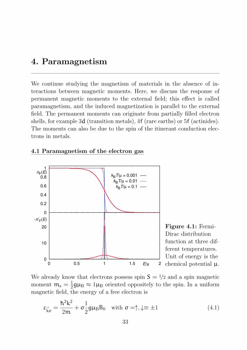
Figure 4.1: Fermi-

Dirac distribution

function at three dif-

ferent temperatures.

Unit of energy is the

chemical potential µ.

We already know that electrons possess spin S = 1/2 and a spin magnetic

moment ms =12gµB ≈ 1µB oriented oppositely to the spin. In a uniform

magnetic field, the energy of a free electron is

εkσ

= h2k2

2m+ σ

1

2gµBB0 with σ =↑, ↓≡ ±1 (4.1)

33

With chemical potential µ, the total energy of the Fermi gas is then

E =∑kσ

εkσnF

(εkσ

)(4.2)

with Fermi-Dirac distribution function (in short, Fermi function)

nF(ε) =1

1 + eε−µkBT

.

This is shown in Figure 4.1. The magnetization is given by

M = −gµB

2V

∑kσ

σnF(εkσ) (4.3)

and the susceptibility is

χ =∂M

∂B0

∣∣∣∣B0=0

= −gµB

2V

∑kσ

σn ′F

( h2k2

2m

)σgµB

2

= −g2µ2

B

4V2∑k

n ′F

( h2k2

2m

)= −

g2µ2B

2V

∑k

n ′F

( h2k2

2m

)(4.4)

∑σ contributes the factor 2. We can now replace the k summation by an

energy integration, ∑k

→∫dεD(ε) ,

using the density of states for one spin direction

D(ε) =1

V

∑k

δ

(ε−

h2k2

2m

)and find

χ = −g2µ2

B

2

∫dεD(ε)n ′F(ε) . (4.5)

For kBT µ, which is typically the case for metals, nF(ε) can be approx-

imated by a Heaviside step function Θ(ε), and therefore −n ′F(ε) as a δfunction: n ′F(ε) ≈ −δ(ε) (see also Figure 4.1). This means

χ =g2µ2

BD(µ)

2=: χPauli . (4.6)

34

This is the so-called Pauli susceptibility which describes the Pauli param-

agnetism. The result is valid not only for free electrons but for any kind of

dispersion if the appropriate density of states D(ε) is inserted. As long as

kBT µ, the result is temperature independent. The Pauli susceptibility

is related to the Landau susceptibility via

χLandau = −1

3χPauli . (4.7)

Thus, the total susceptibility of the free electron gas in three dimensions is

χ = χPauli + χLandau =2

3χPauli . (4.8)

Excursion: Sommerfeld expansion

Integrals of the type∫dEH(E)nF(E) (4.9)

involving the Fermi function nF(E) =(eE−µkBT + 1

)−1often occur in solid

state physics, for example in the internal energy of the electron system

U =∑lkσ

〈nlkσ〉εl(

k) = N

∫dEnF(E)D(E)E (4.10)

where 〈nlkσ〉 is the average occupation of the single particle states l as

function of temperature, given by the Fermi function; D(E) is the density

of states per unit cell. The total particle number can be expressed as

Ne =∑lkσ

〈nlkσ〉 = N

∫dED(E)nF(E) (4.11)

The Sommerfeld expansion can be applied if the function H(E) is multiply

continuously differentiable and integrable and disappears for E → −∞;

then we have (by partial integration)∫∞−∞ dEH(E)nF(E) =

∫∞−∞ dEK(E)

(−dnF

dE

)+[K(E)nF(E)

]∞−∞

=0

(4.12)

where

K(E) =

∫E−∞ dE ′H(E ′) (4.13)

35

is the antiderivative ofH(E). Explicitly, the negative derivative of the Fermi

function is

−dnF

dE=

1

kbT

1

(eE−µkBT + 1)(e

−E−µkBT + 1)

. (4.14)

Examples of this function are shown in Figure 4.1. It is symmetric with

respect to the chemical potential µ and falls exponentially on both sides.

For T → 0 the derivative becomes a δ function. At finite temperatures,

it is only nonzero in a region which grows approximately linearly with

temperature. Therefore, the energy integral needs only to be done in a

small interval around µ, and the function K(E) is expanded in a Taylor

series around µ:

K(E) = K(µ) +

∞∑n=1

1

n!(E− µ)n

dnK(E)

dEn

∣∣∣∣E=µ

(4.15)

Inserting the integral that we want to calculate, we find∫∞−∞ dEH(E)nF(E) =

∫µ−∞ dEH(E) +

∞∑n=1

dn−1H(E)

dEn−1

∣∣∣∣E=µ

∫∞−∞ dE

(E− µ)n

n!

(−dnF

dE

)because

∫∞−∞ dE

(−dnF

dE

)K(µ) =

[− nF(E)K(µ)

]∞−∞ = K(µ)

(4.16)

Thus, the series contains only derivatives of the function we want to in-

tegrate, taken at the chemical potential µ as well as integrals that are

independent of H(E). As −dnFdE

is symmetric around µ, integrals over odd

powers of (E− µ) drop out. With the substitution x = E−µkBT

we have∫∞−∞ dEH(E)nF(E) =

∫µ−∞ dEH(E) +

∞∑n=1

an(kBT)2nd

2n−1H(E)

dE2n−1

∣∣∣∣E=µ

with an =

∫∞−∞ dx

x2n

(2n)!

1

(ex + 1)(e−x + 1)(4.17)

The an can be calculated analytically:

an =(

2 −1

22(n−1)

)ζ(2n) (4.18)

36

with the Riemann zeta function

ζ(x) =

∞∑m=1

1

mx= 1 +

1

2x+

1

3x+ . . .

In particular,

a1 = ζ(2) =π2

6, a2 =

7

4ζ(4) =

7

4

π4

90=

7π4

360

Thus, the expansion up to fourth order in kBT is∫∞−∞ dEH(E)nF(E) =

∫µ−∞ dEH(E)

+π2

6(kBT)

2dH(E)

dE

∣∣∣∣E=µ

+7π4

360(kBT)

4d2H(E)

dE2

∣∣∣∣E=µ

(4.19)

Using the Sommerfeld expansion, we find

Ze =Ne

N=

∫dED(E)nF(E) =

∫µ−∞ dED(E) +

π2

6(kBT)

2D ′(µ) + O(T 4)

U

N=

∫dEnF(E)D(E)E =

∫µ−∞ dED(E)E+

π2

6(kBT)

2(µD ′(µ) +D(µ)

)+ O(T 4)

(4.20)

4.2 Paramagnetism of localized electrons

Now we discuss the paramagnetism of insulators. Here, the electrons that

are responsible for the paramagnetism are strictly localized at fixed lattice

points and produce a permanent magnetic moment there. This picture is

almost ideally realized in rare earths and their compounds; they are often

called 4f systems because of the electron shell that is successively filled.

The neutral rare earth atom has the configuration

[Xe]4fp6s2 ,

i.e. a noble gas configuration of xenon plus 4f and 6s electrons. In the

periodic table, the rare earths start with La (lanthanum) and then add

4f electrons until Lu (lutetium). Usually, the rare earths are trivalent, i.e.

(RE)3+, and they give away the 6s electrons and one 4f electron. The

37

partially filled 4f shell is situated inside the xenon core and is strongly

screened by the fully filled 5s25p6 shells which lie outside the xenon core.

This strongly localizes the magnetic moments of the 4f electrons to their

respective lattice points.

Such a system can be described by a very simple model: We assume that

in volume V , there are N identical independent ions; we only care about

the magnetic moments produced by these ions. We can assume that intra-

atomic correlations are so strong that the localized magnetic moment is

determined by the atomic Hund’s rules. The temperature and field depen-

dence of the magnetization M is essentially an atomic problem.

Figure 4.2: Para-

magnetic local mo-

ments in an exter-

nal magnetic field.

0B

We now assume LS-coupling which is valid for not too strong spin-orbit

coupling. The distances between different LS multiplets are so large that

transitions among them are improbable and we can assume that quantum

numbers L and S belonging to the squares L2 and S2 of the total angular

momentum and total spin quantum numbers are good quantum numbers.

The magnetic momentmj of the ion at lattice site j is given by

mj = −

µB

h

(Lj + 2

Sj)= −

µB

h

(Jj +

Sj)

. (4.21)

In the following, we disregard the minus sign in the definition of the mag-

netic moment. The model Hamiltonian is

H =

N∑j=1

(H

(j)0 +H

(j)SO −

mj ·

B0

)=

N∑j=1

H(j)1 (4.22)

As we are restricting the discussion to a single LS multiplet, H(j)0 which

determines the coarse structure of the terms is not important. The spin

orbit coupling of each ion H(j)SO determines the fine structure of the terms.

The last expression in the bracket represents the Zeeman energy, and its

relative strength in comparison to H(j)SO is decisive for the calculation of the

magnetization

M = n〈m〉 with n =N

V.

38

Here, the bracket 〈. . . 〉 means quantum mechanical expectation value and

thermal averaging; in general

〈A〉 = 1

ZTr(Ae−βH

)with canonical partition function Z = Tr

(e−βH

)= ZN1 which factorizes

for the model (4.22) into a product of single-particle partition functions

Z1 = Tr(e−βH1

)because the moments do not interact. β is the inverse temperature β = 1

kBT.

If we now apply a homogeneous magnetic field

B0 in z direction, the x and

y components of the magnetization vanish, and we find for Mz =M

M = n1

Z1Tr(me−βH1

)= kBTn

∂

∂B0lnZ1 (4.23)

Determining the single-particle partition function Z1 already solves the

problem; however, we can calculate the trace only for particular situations.

M is influenced by the thermal energy kBT , by the spin-orbit interaction

HSO = Λ(γ,LS)

L ·

S (γ stands for other quantum numbers) and the

magnetic field Hz = −µB h (Jz+Sz)B0. Only if there are orders of magnitude

between these three terms can the partition function Z1 be determined

easily.

Weak spin-orbit interaction.- This is the case h2Λ(γ,LS)

L kBT .

Furthermore, we have to distinguish small and large field compared to the

temperature of interest.

a) h2Λ(γ,LS)

L kBT ,µBB0

We can assume that we have the so-called normal Zeeman effect

EγLSJMJ= E

(0)γLS − (ML + 2MS)µBB0 ,

and all terms of the LS multiplet are occupied with almost equal proba-

bility. ML and MS are “still good” quantum numbers, but J is not a good

quantum number. E(0)γLS are eigenenergies of H0 without field and without

spin-orbit coupling. We calculate the partition function in energy represen-

tation

Z1 = e−βE

(0)γLS

+L∑ML=−L

+S∑MS=−S

eβµBB0(ML+2MS) (4.24)

39

We focus on the lowest LS multiplet as the prefactor will be very small for

the higher ones. With the notation b = βµBB0 > 0 we calculate

+L∑ML=−L

ebML = ebL2L∑n=0

(e−b)n = ebL1 − e−b(2L+1)

1 − e−b

= ebLeb/2 − e−

b/2−2Lb

eb/2 − e−b/2=eb(L+

1/2) − e−b(L+1/2)

eb/2 − e−b/2

=sinh

(b(L+ 1/2)

)sinh

(b2

) (4.25)

The same calculation also gives

+S∑MS=−S

ebMS =sinh

(b(2S+ 1)

)sinhb

. (4.26)

Therefore, the partition function is

Z1 = e−βE

(0)γLS

sinh(βµBB0(L+ 1/2)

)sinh

(12βµBB0

) sinh(βµBB0(2S+ 1)

)sinh(βµBB0)

. (4.27)

With the magnetization of a paramagnet (4.23), we now need to differen-

tiate the partition function with respect to the field:

∂

∂B0lnZ1 =

1

Z(L)1

∂Z(L)1

∂B0+

1

Z(S)1

∂Z(S)1

∂B0. (4.28)

We do the first term explicitly:

1

Z(L)1

∂Z(L)1

∂B0=

sinh(b2

)sinh

(b(L+ 1/2)

)sinh(b2

)βµB(L+ 1/2) cosh

(b(L+ 1/2)

)sinh2

(b2

) −

−sinh

(b(L+ 1/2)

)12βµB cosh

(b2

)sinh2

(b2

) = βµB(L+ 1/2) coth

(b(L+ 1/2)

)−

1

2βµB coth

(b2

)(4.29)

Now we introduce a function which is central to the theory of magnetism,

the Brillouin function:

BD(x) =2D+ 1

2Dcoth

(2D+ 1

2Dx

)−

1

2Dcoth

(x

2D

)(4.30)

40

0

0.5

1

0 5 10

BD

(x)

x

D = 1⁄2

D = 1D = 3

⁄2

D = ∞

Figure 4.3: Bril-

louin function

BD(x) as function

of x for several pa-

rameters D.

Using this function, we can write the magnetization of Eq. (4.23) in the

form

M(T ,B0) = nµB

[LBL(βµBB0L) + 2SBS(2βµBB0S)

](4.31)

A few general properties of the Brillouin function are:

1. D = 1/2: In this special case,

B1/2(x) = tanh x .

2. D→∞: In this limit, the Brillouin function reduces to the Langevin

function L(x):

BD→∞(x) = L(x) = coth x−1

x.

This function appears in the classical treatment of paramagnetism if

the quantization of the orbital angular momentum is neglected (mo-

ments can assume any angle in space).

3. Small x: By expanding coth x, one finds

BD(x) =D+ 1

3Dx−

D+ 1

3D

2D2 + 2D+ 1

30D2x3 + . . . , (4.32)

and, in particular

BD(0) = 0 .

Due to this property, according to (4.31), the magnetization of a para-

magnet is zero if either B0 = 0 or T =∞. Physically, this means that

a paramagnet does not possess spontaneous magnetization.

41

4. BD(−x) = −BD(x): This means that if the direction of the magnetic

field is reversed, the direction of the magnetization is also reversed.

5. limx→∞BD(x) = 1: The magnetization shows saturation for B0 →∞ or

for T → 0. This means that all the moments are oriented parallel to the

field:M→M0 = nµB(L+2S). The high temperature behavior of the

magnetization is interesting. With the precondition we are discussing

here h2Λ(γ,LS) µBB0 kBT or βµBB0 1, the argument

of the Brillouin function is small, and the expansion (4.32) can be

terminated after the linear term:

M ≈nµ0µ

2B

3kBTB0

[L(L+ 1) + 4S(S+ 1)

](4.33)

The susceptibility

χ = µ0

(∂M

∂B0

)T

then shows a characteristic 1T

behavior, which is called the Curie law:

χ(T) =C1

T. (4.34)

C1 is the so-called Curie constant which is given by

C1 =nµ0µ

2B

3kB

[L(L+ 1) + 4S(S+ 1)

].

A purely classical calculation would have given a similar high-temperature

behavior:

χcl(T) =Ccl

T, Ccl =

nµ0µ2

3kB, (4.35)

where µ is the magnetic moment. In analogy, one therefore defines

µeff = µBpeff , peff =√L(L+ 1) + 4S(S+ 1) (4.36)

with the effective number of Bohr magnetons peff .

b) So far, we assumed that both thermal energy and field energy are large

compared to the spin-orbit interaction. If we now allow the spin-orbit cou-

pling energy to be of the same order of magnitude as the magnetic energy

but still smaller than the thermal energy

h2Λ(γ,LS),µBB0 kBT

42

the calculation becomes more complicated because the spin-orbit coupling

term enters the partition function. However, after considering all terms,

the result for the magnetization is

M =nµ0µ

2B

3kBTB0

[L(L+ 1) + 4S(S+ 1)

](4.37)

which is the same as the high temperature limit of case a), Eq. (4.33).

Strong spin-orbit interaction.- h2Λ(γ,LS) kBT ,µBB0. This case is

different; it is often discussed as Langevin paramagnetism and occurs for

4f systems in moderate fields. Rather than a uniform distribution over the

fine structure terms of the LS multiplets, only the lowest term is occupied

to a certain degree. J is still a “good” quantum number, and non-diagonal

terms of Sz only play a marginal role; this region is called the anomalous

Zeeman effect, and the energies are

EγLSJMj= E

(0)γLSJ + gJ(L,S)MJµBB0 (4.38)

with Lande g factor from Eq. (2.21). Then, the partition function is

Z1 = e−βE

(0)γLSJ

+J∑MJ=−J

e−βgJMJµBB0 . (4.39)

Only the energetically most favorable J value, according to Hunds’ third

rule, has to be taken into account. The partition function is calculated as

shown above for weak spin-orbit coupling, Eq. (4.27):

Z1 = e−βE

(0)γLSJ

sinh(βgJµBB0(J+ 1/2)

)sinh

(12βgJµBB0

) (4.40)

This gives us the magnetization

M =M0BJ(βgJJµBB0

)(4.41)

with saturation magnetization

M0 = nJgJµB . (4.42)

As before, the susceptibility follows from differentiating with respect to

the field B0. The high temperature behavior is again the Curie law (for

βµBB0 1)

χ =C

Twith C = nµ0

p2eff

3kBµ2

B (4.43)

43

where in the Curie constant C now a different effective magneton number

is found:

peff = gJ√J(J+ 1) . (4.44)

The Curie law is experimentally very well confirmed, and the order of

magnitude of χLangevin is normally much larger than the Pauli magnetism

of the conduction electrons:

χPauli

χLangevin=

9

2

1

g2JJ(J+ 1)

kBT

εF(4.45)

44

5. Exchange interaction

The dipole interaction between the magnetic moments of the electrons is

much too weak for supporting magnetic order of materials at high temper-

atures. For explaining the observed magnetism, we need to find a strong

interaction between the electrons. We might think that an interaction de-

pending explicitly on the spin (the magnetic moments) of the electrons is

needed; no such interaction is known though. In 1928, Werner Heisenberg

realized that the responsible interaction is the Coulomb repulsion between

electrons; this is a strong interaction but does not explicitly depend on

the spin. Spin selectivity is due to quantum mechanics, in particular the

Pauli principle: Two electrons with parallel or antiparallel spin behave dif-

ferently even though the fundamental interaction is the same; the spatial

wave function ψ(r1,

r2) has to be antisymmetric and symmetric, respec-

tively. One consequence is that two electrons with parallel spin cannot be

in the same place. In order to discuss how the Coulomb interaction term

leads to an exchange interaction of the spins, we first write this interaction

in second quantization; we will introduce this very useful representation

first.

5.1 Occupation number representation for fermions

So far, we have discussed the Hamiltonian in so-called first quantization:

H = H0+H1 ,H0 =

Ne∑i=1

hi =

Ne∑i=1

P2i

2m+

Ne∑i=1

V(ri) ,H1 =

∑i<j

u(ri−

rj)

(5.1)

where u(ri −

rj) is either the bare Coulomb potential

u(ri −

rj) =

e2

|ri −

rj|

(5.2)

or an effective, screened interaction. First quantization implies that the an-

tisymmetry of the wave function has to be taken into account by working

45

with Slater determinants which is rather cumbersome. Therefore, many-

body calculations in solid state theory are usually performed in so-called

second quantization, using the occupation number representation.

Slater determinant

Let’s assume that we can solve the single particle problem exactly, i.e. for

electron i we have

hi|kα〉(i) = εkα |kα〉(i) (5.3)

or in position representation

hiϕkα(ri) =

( p2i

2m+ V(

ri)

)ϕkα(

ri) = εkαϕkα(

ri) (5.4)

with a complete set of single particle quantum numbers kα = (l,

k,σ)of Bloch states. The Pauli principle now implies that only the part of the

product space of Ne single particle Hilbert spaces is realized which consists

of the particle indices of totally antisymmetric wave functions. A basis of

the Ne particle Hilbert space are the Slater determinants which we can

compose of single particle states as follows:

|ψk1,··· ,kNe(1 · · ·Ne)〉 =1√Ne!

∑P∈SNe

(−1)χP |kP(1)〉(1) · · · |kP(Ne)〉(Ne)

=1√Ne!

det

|k1〉(1) · · · |k1〉(Ne)...

...

|kNe〉(1) · · · |kNe〉(Ne)

=1√Ne!

det(|kα〉(i)

)(5.5)

where P are the elements of the permutation group SNe ofNe elements, and

χP is the character of the permutation (number of transpositions, which

lead to the permutation). The product state

|k1〉(1)|k2〉(2) · · · |kNe〉(Ne)

means that particle 1 is in state k1, particle 2 in state k2 and so on; but as

the particles are not distinguishable, it has to be irrelevant which particle is

in state k1,k2 etc. Therefore, we have to sum over all possible permutations.

The Slater determinants are a suitable basis for the Ne particle Hilbert

space HA(Ne), even if not all states of this Hilbert space correspond to a

single Slater determinant.

46

Fock space

The basis of HA(Ne) which is described by Slater determinants can also be

written down in occupation number representation by writing down how

many of the indistinguishable Ne particles are in state kα; however, the

sum over all occupation numbers has to be Ne. We can get rid of this

restriction if we do not work in the Ne particle Hilbert space but instead

in Fock space

HA,Fock = HA(0)⊕HA(1)⊕ · · · ⊕HA(Ne)⊕ · · · (5.6)

which is defined as direct sum over the Hilbert spaces for all possible par-

ticle numbers. If we allow an arbitrary number of (identical) particles in

the Hilbert space, then this product space is called Fock space. We can

now define operators that “ascend” and “descend” between segments of

Fock space with different particle numbers. These operators create and

annihilate particles; therefore, they are called creation and annihilation

operators. They play a central role in many serious calculations within

quantum mechanics. Fock space is always explicitly or implicitly used for

grand canonical treatments. In the following, we note the most important

relations for fermions and bosons; therefore, we use N for the number of

particles.

Starting point is the representation of N particle states. Let’s assume a

discrete, ordered single particle basis is given: |1〉, |2〉, . . . , where i in |i〉stands for a set of single particle quantum numbers (l

kσ)i. The normaliza-

tion is 〈i|j〉 = δij. All N particle states can be represented by superposition

of

P±(|r1〉|r2〉 . . . |rN〉

)(5.7)

where P+ symmetrizes for bosons and P− antisymmetrizes for fermions.

Explicitly, we have

P−(|r1〉|r2〉 . . . |rN〉

)=

1√N!

∑P∈SN

(−1)P|rP(1)〉|rP(2)〉 . . . |rP(N)〉 (5.8)

and

P+(|r1〉|r2〉 . . . |rN〉

)=

1√N!n1!n2! . . .

∑P∈SN

|rP(1)〉|rP(2)〉 . . . |rP(N)〉 (5.9)

where P runs over all permutations and ni is the number of single particle

states |i〉 in the product.

47

An equivalent characterization of the (basis) states is possible in occupation

number representation:∣∣n⟩ ≡ |n1,n2, . . . 〉 := P±(|1〉 . . . |1〉︸ ︷︷ ︸n1 times

|2〉 . . . |2〉︸ ︷︷ ︸n2 times

. . .)

(5.10)

(Obviously, for fermions we have ni ∈ 0, 1).∣∣n⟩ thus stands for a com-

plete set of occupation numbers for all single particle states.

A further step for the efficient representation is the introduction of particle

creation and annihilation operators: c†i , ci. We do this for fermions here

and cite the result for bosons below. We define ci and c†i by their effect on

the basis states as follows:

ci∣∣n⟩ = ci| . . .ni . . . 〉 = (−1)

∑i−1j=1 nj | . . . (ni − 1) . . . 〉

c†i∣∣n⟩ = c†i | . . .ni . . . 〉 = (−1)

∑i−1j=1 nj | . . . (ni + 1) . . . 〉 (5.11)

Concerning the notation, c†i is indeed the adjunct operator for ci:⟨m∣∣ci∣∣n⟩ =

(−1)

∑j<i nj, if mi = ni − 1 ,mj = nj for j 6= i ,

0, otherwise⟨n∣∣c†i∣∣m

⟩=

(−1)

∑j<imj, if ni = mi + 1 ,nj = mj for j 6= i ,

0, otherwise(5.12)

Remark: ci maps totally antisymmetric N particle states to totally anti-

symmetric (N− 1) particle states; c†i acts “in the opposite way”: Creation

and annihilation, respectively.

For the particle operators the important anticommutation relations are

valid:

[ci, cj]+ = cicj + cjci = 0 (5.13)

and also

[c†i , c†j ]+ = c†ic

†j + c

†jc†i = 0 (5.14)

Verification: we assume i < j (otherwise, the labels can be exchanged, i = jis obvious):

cicj∣∣n⟩ = ci(−1)νj | . . . (nj − 1) . . . 〉

= (−1)νi+νj | . . . (ni − 1) . . . (nj − 1) . . . 〉cjci∣∣n⟩ = cj(−1)νi | . . . (ni − 1) . . . 〉

48

= (−1)νj−1+νi | . . . (ni − 1) . . . (nj − 1) . . . 〉 (5.15)

Here we abbreviated νi =∑i−1j=1 nj. Thus, the second equation of (5.15) has

an extra minus sign, and if we add both equations, we find cicj+ cjci = 0.

Furthermore,

[ci, c†j ]+ = δij (5.16)

Justification: We assume i < j (otherwise, we again relabel); as before, we

find

cic†j

∣∣n⟩ = (−1)νi+νj | . . . (ni − 1) . . . (nj + 1) . . . 〉c†jci

∣∣n⟩ = (−1)νj−1+νi | . . . (ni − 1) . . . (nj + 1) . . . 〉 (5.17)

i.e. for i 6= j ci and c†j anticommute. Now let i = j:

cic†i

∣∣n⟩ =

∣∣n⟩, if ni = 0 ,

0, if ni = 1 ,

c†ici∣∣n⟩ =

0, if ni = 0 ,∣∣n⟩, if ni = 1 ,

(5.18)

From the sum of these two equations, we obtain

(cic†i + c

†ici)|n〉 =

∣∣n⟩y [ci, c†i ]+ = 1 .

If we now define the vacuum as

|0〉 := |00 . . . 0 . . . 〉 (5.19)

then we have∣∣n⟩ = (c†1)n1(c†2)

n2 . . . |0〉, (5.20)

so that for N particle states, we obtain

c†r1c†r2

. . . c†rN |0〉, (5.21)

Therefore, we have the correspondence, for example for two particles∣∣ψk1k2(12)⟩=

1√2

∣∣∣∣|k1〉(1) |k1〉(2)|k2〉(1) |k2〉(2)

∣∣∣∣ ↔ c†1c†2|0〉 (5.22)∣∣ψk1k2(12)

⟩= −

∣∣ψk2k1(12)⟩↔ c†2c

†1|0〉 = −c†1c

†2|0〉 (5.23)

49

Both for the Slater determinant in first quantization and in second quan-

tization, the antisymmetry of the wave function is guaranteed.

In particular for fermions, this has the consequence

c†1c†1|0〉 = −c†1c

†1|0〉 = 0 ,

two fermions cannot have the same quantum numbers.

For bosons, we briefly note the definitions

ci| . . .ni . . . 〉 =√ni| . . . (ni − 1) . . . 〉

c†i | . . .ni . . . 〉 =√ni + 1| . . . (ni + 1) . . . 〉 (5.24)

as well as the commutation relations

[ci, cj] = [c†i , c†j ] = 0

[ci, c†j ] = δij (5.25)

Particle number operator

From the anticommutation (commutation) relations, we can also conclude

that the operator ni = c†ici (for bosons: ni = b

†ibi) is the particle number

operator. For fermions, we have

ni| . . . (ni = 0) . . . 〉 = c†ici| . . . (ni = 0) . . . 〉 = 0

ni| . . . (ni = 1) . . . 〉 = c†icic†i | . . . (ni = 0) . . . 〉

= c†i(1 − c†ici

)| . . . (ni = 0) . . . 〉 = | . . . (ni = 1) . . . 〉 .

(5.26)

For bosons,

ni(b†i)N

|0〉 = N(b†i)N

|0〉 ,as can easily been shown recursively.

Change of basis

If we change from one single particle basis |i〉 to another, |i〉, by inserting

a unit operator

c†j |0〉 ≡ |j〉 =∑i

|i〉〈i|j〉 =∑i

〈i|j〉 c†i |0〉 , (5.27)

the operators ci turn into operators cj according to

c†j =∑i

〈i|j〉 c†i , cj =∑i

〈j|i〉 ci . (5.28)

50

Operators in second quantization

So far, we have only considered a discrete single particle basis |i〉. We will

now define field operators Φ(x) over the single particle states corresponding

to the position operator, and analogously field operators ck

that correspond

to the momentum operator:

Φ(x) =

∑i

〈x|i〉ci

ck

=∑i

〈

k|i〉ci =∫d3x〈

k|x〉∑i

〈x|i〉ci =1

(2π)3/2

∫d3x e−i

k·xΦ(

x)

(5.29)

Here, the unit operator 1 =∫d3x |

x〉〈x| was introduced. Furthermore,

Φ(x) =

∫d3k∑i

〈x|

k〉〈

k|i〉ci =∫d3k〈x|

k〉ck=

1

(2π)3/2

∫d3k ei

k·xc

k

(5.30)

Field operators corresponding to the position operator Φ(x) (Φ†(

x)) an-

nihilate (create) a particle at positionx (while annihilation/creation op-

erators ci, c†i do this for particles in a certain single particle state). The

anticommutation relations[Φ(

x), Φ(

y)]+

=[Φ†(

x), Φ†(

y)]+= 0,[

Φ(x), Φ†(

y)]+

=∑i,j

〈x|i〉〈j|y〉[ci, c

†j

]+

=∑i

〈x|i〉〈i|y〉 = 〈x|y〉 = δ3(x−

y) (5.31)

and analogously for ck

are valid.

Remark. For systems with a finite volume V one defines Φ(x) and c

k

as above;x then varies continuously over V and

k is quantized with cor-

responding volume d3k = (2π)3

V. Transformation from Φ(

x) to c

kis done

using 〈x|k〉 = 1√V

eikx. The (anti-) commutation relations are valid as noted

above, and the δ symbol for operators ck, c†

kbecomes a Kronecker delta.

Representation of states

51

Let |ψ〉 be an N particle state; then we can write |ψ〉 as

|ψ〉 = 1

N!

∫d3x1 . . .d3xNψ(

x1,

x2, . . . ,

xN)Φ

†(x1) . . . Φ†(

xN)|0〉 (5.32)

with a function ψ(x1,

x2, . . . ,

xN) which is chosen totally (anti-)symmetric

without loss of generality. We remember that

P−(|x1〉|

x2〉 . . . |

xN〉)=: |

x1

x2 . . .

xN〉 = Φ†(

x1)Φ

†(x2) . . . Φ†(

xN)|0〉

(5.33)

Apparently, the function ψ(x1,

x2, . . . ,

xN) is the wave function in second

quantization.

We can also see by applying (anti-) commutation rules, that

〈y1y2 . . .

yN|ψ〉 = ψ(

y1,

y2, . . . ,

yN):

〈y1y2 . . .

yN|ψ〉 =

1

N!

∫d3x1 . . .d3xNψ(

x1,

x2, . . . ,

xN)×

×〈0|Φ(yN) . . . Φ(

y1)Φ

†(x1) . . . Φ†(

xN)|0〉

= ψ(y1,

y2, . . . ,

yN) (5.34)

This presents the explicit relationship between first and second quantiza-

tion.

So far, we have only considered one species of particles. We will for example

consider interactions between electrons (fermions) and phonons (bosons).

The corresponding states will then be created by products of fermionic and

bosonic creation operators, for example

c†k1c†k2b†q1b†q2b†q3|0〉 (5.35)

as a state of two fermions and three bosons with momenta

k1,

k2, andq1,

q2,

q3. Here, different fermions anticommute, and bosons among each

other as well as bosons and fermions commute.

Operators in occupation number representation

In the description of many particle systems, so-called one particle and two

particle operators appear. In first quantization, we can write a one particle

operator for an Ne particle system as

A(1) =

Ne∑i=1

A(1)(ri) . (5.36)

52

It is added up from contributions, each of which is only acting on one of the

Ne particles. Examples are the kinetic energy and the external potential of

the single particle Hamiltonian, the current operator or the particle density

operator. Two particle operators in first quantization are of the form

A(2) =1

2

∑i 6=jA(2)(

ri,

rj) . (5.37)

All addends simultaneously act on two different particles. An example is

the Coulomb interaction. Now, we express the one particle operator by

creation and annihilation operators by introducing the unit operators 1 =∑α |kα〉(i) (i)〈kα|:

A(2) =

Ne∑i=1

∞∑α=1

|kα〉(i) (i)〈kα|A(1)(ri)

∞∑β=1

|kβ〉(i) (i)〈kβ|

=

∞∑α,β=1

〈kα|A(1)(r)|kβ〉

Ne∑i=1

|kα〉(i) (i)〈kβ| (5.38)

Here we used that the matrix element of A(1) with respect to the single

particle states is not anymore dependent on the particle index:

(i)〈kα|A(1)(ri)|kβ〉(i) =

∫d3riϕ

∗kα(ri)A

(1)(ri)ϕkβ(

ri) = 〈kα|A(1)(

r)|kβ〉

(5.39)

We have

Ne∑i=1

|kα〉(i) (i)〈kβ| = c+kαckβ (5.40)

because the operator |kα〉(i) (i)〈kβ|, applied to an Ne particle state only

gives a non-zero result if the one particle state kβ is contained in the

manyparticle state; in this case, the state |kβ〉 in this manyparticle state is

replaced by |kα〉; this corresponds to the annihilation of a particle in the

state kβ and the creation of a particle in the state kα.

Thus, the single particle operator in occupation number representation is

A(1) =

∞∑α,β=1

A(1)kα,kβ

c†kαckβ with A(1)kα,kβ

= 〈kα|A(1)(r)|kβ〉 (5.41)

53

The one particle operator is expressed as a linear combination over all

possible pairs of creation and annihilation operators, with matrix elements

of the single particle operator with respect to the single particle states as

coefficients. Correspondingly, we have for the two particle operator, if we

insert unit operators:

A(2) =1

2

∑i 6=j

∑α,β,γ,δ

|kα〉(i)|kβ〉(j) (i)〈kα| (j)〈kβ|A(2)(ri,

rj)|kγ〉(j)|kδ〉(i) (j)〈kγ| (i)〈kδ|

=1

2

∑α,β,γ,δ

A(2)kαkβ,kγkδ

∑i 6=j

|kα〉(i)|kβ〉(j) (j)〈kγ| (i)〈kδ|

(5.42)

with the two particle matrix element

A(2)kαkβ,kγkδ

= (i)〈kα| (j)〈kβ|A(2)(ri,

rj)|kγ〉(j)|kδ〉(i)

=

∫d3rid

3rjϕ∗kα(ri)ϕ

∗kβ(rj)A

(2)(ri,

rj)ϕkγ(

rj)ϕkδ(

ri) (5.43)

which is again independent of the particle indices because in the calculation

of the matrix element in position representation, there is an integral over

these indices. If we apply the operator∑i 6=j |kα〉(i)|kβ〉(j) (j)〈kγ| (i)〈kδ| on

a manybody state we only obtain something nonzero if in this many body

state, the single particle states kγ and kδ are occupied. In this case the

operator replaces these states by kα and kβ; then, in the manybody state

kγ, kδ are unoccupied and kα, kβ are occupied; this corresponds to∑i 6=j

|kα〉(i)|kβ〉(j) (j)〈kγ| (i)〈kδ| = c†kαc†kβckγckδ (5.44)

Thus, the two particle operatorA(2) is in occupation number representation

A(2) =1

2

∑α,β,γ,δ

A(2)kαkβ,kγkδ

c†kαc†kβckγckδ

A(2)kαkβ,kγkδ

=

∫d3rid

3rjϕ∗kα(ri)ϕ

∗kβ(rj)A

(2)(ri,

rj)ϕkγ(

rj)ϕkδ(

ri) (5.45)

All operators become linear combinations of creation and annihilation op-

erators with coefficients which are given by the matrix element of the cor-

responding operator with respect to the single particle states.

54

The operators can also be expressed using the representation of free field

operators:

A(1) =

∫d3r Φ†(

r)A(1)(

r)Φ(

r)

A(2) =1

2

∫d3rd3r ′ Φ†(

r)Φ†(

r ′)A(2)(

r,

r ′)Φ(

r ′)Φ(

r) (5.46)

This can be checked by introducing the expansion of the field operators

in a single particle basis. The name second quantization is now due to the

fact that in these relationships, also the wave functions are replaced by

operators.

Especially the Hamiltonian (5.1) can now be written in occupation number

representation:

H = H0 +H1 =∑α

εkαc†kαckα+

1

2

∑α,β,γ,δ

ukαkβ,kγkδc†kαc†kβckγckδ (5.47)

where the single particle basis of the single particle Hamiltonian was used.

We have

ukαkβ,kγkδ =

∫d3rd3r ′ϕ∗kα(

r)ϕ∗kβ(

r ′)u(

r−

r ′)ϕkγ(

r ′)ϕkδ(

r) (5.48)

The use of a different single particle basis is also possible; however, the

single particle component of H is then not diagonal anymore.

5.2 Direct ferromagnetic exchange interaction

The Coulomb interaction is

HCoulomb =1

2

1

4πε0

∫d3r1d

3r2ρ(

r1)ρ(

r2)∣∣r1 −r2∣∣ (5.49)

In second quantized notation, ρ(r) is the operator of the charge density

ρ(r) = −e

∑σ

ψ†σ(r)ψσ(

r)

with spin orientation σ =↑, ↓ and the field operator ψσ(r). This operator

satisfies the anticommutation relations[ψσ1(

r1),ψ

+σ2(r2)]+≡ ψσ1(

r1)ψ

+σ2(r2) +ψ

+σ2(r2)ψσ1(

r1) = δσ1σ2δ(

r1 −

r2)[

ψσ1(r1),ψσ2(

r2)]+= 0

[ψ+σ1(r1),ψ

+σ2(r2)]+= 0

55

(5.50)

as it is a Fermionic field. We find

HCoulomb =1

2

1

4πε0

∫d3r1d

3r2∑σ1σ2

ψ†σ1(r1)ψσ1(

r1)

e2∣∣r1 −r2∣∣ψ†σ2(r2)ψσ2(r2)

=1

2

1

4πε0

∫d3r1d

3r2∑σ1σ2

ψ†σ1(r1)ψ

†σ2(r2)

e2∣∣r1 −r2∣∣ψσ2(r2)ψσ1(r1)

+1

2

1

4πε0

∫d3r1∑σ1

e2∣∣r1 −r1∣∣ψ†σ1(r1)ψσ1(r1)

(5.51)

The last singular term is unphysical; in fact, the field operators should

be written in normal order (ψ†ψ†ψψ) from the start. ψ can be expanded

into any orthonormal set of single particle wave functions. A set of Wannier

functions, i.e. orthonormal functions φRm

(r) localized at the ion position

R is advantageous; m includes all orbital quantum numbers except for the

spin σ. We also introduce spinors

χ↑ =

(1

0

),χ↓ =

(0

1

)which are eigenvectors of

sz =1

2σz =

1

2

(1 0

0 −1

)with eigenvalues ±1

2 . Then the field operator is

ψσ(r) =

∑Rm

aRmσ

φRmχσ (5.52)

with Fermionic annihilation operators aRmσ

which satisfy [aRmσ

,a†Rmσ

]+ =

δRR ′δmm ′δσσ ′ etc. The Coulomb interaction becomes

HCoulomb =1

2

∑R1m1

· · ·∑R4m4

∫d3r1d

3r2φ∗R1m1

(r1)φ

∗R2m2

(r2)

e2

4πε0|r1 −

r2|×

× φR3m3

(r2)φ

R4m4(r1)∑σ1σ2

χ†σ1χ†σ2χσ2χσ1a

†R1m1σ1

a†R2m2σ2

aR3m3σ2

aR4m4σ1

56

(5.53)

The scalar product of the spinors are simply χ†σ1χσ1 = χ†σ2χσ2 = 1. We

define the integral⟨

R1m1,

R2m2

∣∣∣ e2

4πε0|r1 −

r2|

∣∣∣R3m4,

R4m4

⟩:=∫

d3r1d3r2φ

∗R1m1

(r1)φ

∗R2m2

(r2)

e2

4πε0|r1 −

r2|φR3m3

(r2)φ

R4m4(r1) (5.54)

and obtain

HCoulomb =1

2

∑R1m1

· · ·∑R4m4

⟨

R1m1,

R2m2

∣∣∣ e2

4πε0|r1 −

r2|

∣∣∣R3m4,

R4m4

⟩×

×∑σ1σ2

a†R1m1σ1

a†R2m2σ2

aR3m3σ2

aR4m4σ1

(5.55)

5.2.1 On-site Coulomb interaction

We first consider the contribution of

R1 =

R2 =

R3 =

R4 ≡

R and drop

the index

R where it doesn’t create confusion. In general, the quantum

numbers m1, . . . ,m4 in the integral⟨m1,m2

∣∣ e2

4πε0|r1−

r2|

∣∣m3,m4

⟩can all be

different and still lead to a nonzero integral. However, in treating HCoulomb

as a perturbation, a nonzero first-order contribution requires a pairing of

creation and annihilation operators a†, a for each orbital. This requires

m1 = m4 and m2 = m3 or m1 = m3, m2 = m4. This leads to the direct

Coulomb integrals

Km1m2:=⟨m1,m2

∣∣∣ e2

4πε0|r1 −

r2|

∣∣∣m2,m1

⟩=

∫d3r1d

3r2|φm1(r1)|

2 e2

4πε0|r1 −

r2|

|φm2(r2)|

2 (5.56)

and the exchange integrals

Jm1m2:=⟨m1,m2

∣∣∣ e2

4πε0|r1 −

r2

∣∣∣m1,m2

⟩=

∫d3r1d

3r2φ∗m1(r1)φ

∗m2(r2)

e2

4πε0|r1 −

r2|φm1(

r2)φm2(

r1) , (5.57)

57

so-called because m1 and m2 are exchanged in the last factor compared to

the direct integrals. To first order we obtain

HCoulomb ≈1

2

∑R

∑m1m2

∑σ1σ2

(Km1m2a

†Rm1σ1

a†Rm2σ2

aRm2σ2

aRm1σ1

+ Jm1m2a†Rm1σ1

a†Rm2σ2

aRm1σ2

aRm2σ1

)(5.58)

(double counting of contributions from m1 = m2 and σ1 = σ2 is not a

problem because the terms contain aRm1σ1

aRm1σ1

= 0). Therefore

HCoulomb ≈1

2

∑R

∑m1m2

∑σ1σ2

(Km1m2a

†Rm1σ1

aRm1σ1

a†Rm2σ2

aRm2σ2

− Jm1m2a†Rm1σ1

aRm1σ2

a†Rm2σ2

aRm2σ1

)+ irrelevant potential terms

(5.59)

We now define the number operators nRm

:=∑σ a†Rmσ

aRmσ

and the spin

operators sαRm

:=∑σσ ′ a

†Rmσ

12σασσ ′a

Rmσ ′with Pauli matrices σα, α =

x,y, z. After some algebra,∑σ1σ2

a†Rm1σ1

aRm1σ2

a†Rm2σ2

aRm2σ1

=1

2nRm1nRm2

+ 2szRm1szRm2

+ s+Rm1

s−Rm2

+ s−Rm1

s+Rm2

=1

2nRm1nRm2

+ 2sRm1· sRm2

(5.60)

Therefore, we obtain

HCoulomb ≈∑R

1

2

∑m1m2

(Km1m2 −

1

2Jm1m2

)nRm1nRm2

− 2Jm1m2

sRm1· sRm2

. (5.61)

The first term is them site Coulomb interaction. From the definition (5.56),

we can read off immediately that Km1m2 > 0. To show that Jm1m2 > 0, we

use the Fourier transform

1

|r1 −

r2|

=

∫d3k

(2π)3ei

k·(r1−

r2)

4π

k2. (5.62)

58

Then,

Jm1m2 =

∫d3k

(2π)3

e2

ε0k2

∫d3r1φ

∗m1(r1)φm2(

r1)e

ik·r1︸ ︷︷ ︸

=:I(k)

∫d3r2φm1(

r2)φ

∗m2(r2)e

−ik·r2︸ ︷︷ ︸

=:I∗(k)

=

∫d3k

(2π)3

e2

ε0k2|I(

k)|2 > 0 .

(5.63)

We also show that Km1m2 > Jm1m2:

Km1m2 − Jm1m2 =1

2

(Km1m2 + Km2m1 − Jm1m2 − Jm2m1

)=

1

2

∫d3r1d

3r2e2

4πε0|r1 −

r2|

[φ∗m1

(r1)φ

∗m2(r2) − φ

∗m2(r1)φ

∗m1(r2)]︸ ︷︷ ︸

=:f(r1,

r2)

×

×[φm2(

r2)φm1(

r1) − φm1(

r2)φm2(

r1)]︸ ︷︷ ︸

=:f∗(r1,

r2)

=1

2

∫d3r1d

3r2e2

4πε0|r1 −

r2|

|f(r1,

r2)|

2 > 0 .

(5.64)

Therefore, the corrected Coulomb term Km1m2 −12Jm1m2 > 0 is reduced

but still repulsive. The new finding is a spin-spin interaction of the form

−Jm1m2

sRm1· sRm2

with Jm1m2 > 0. This interaction prefers parallel alignment of the spins,

i.e. it is a ferromagnetic interaction. Thus, we have derived the first Hund’s

rule: The total spin of electrons in a partially filled shell of one ion tends

to be maximal.

Note that all terms containing Jm1m2 are quantum mechanical in origin;

they appear because we have written the density ρ = −eψ†ψ as a bilinear

form in the field operator which made unconventional pairings of the or-

bital indices possible. There is no analogy in classical physics. For a single

59

relevant orbital φ(r), we get

HCoulomb ≈1

2

∑R

∫d3r1d

3r2φ∗(

r1)φ

∗(r2)

e2

4πε0|r1 −

r2|φ(

r2)φ(

r1)×

×∑σ1σ2

a†Rσ1a†Rσ2aRσ2aRσ1

=1

2

∑R

∫d3r1d

3r2φ∗(

r1)φ

∗(r2)

e2

4πε0|r1 −

r2|φ(

r2)φ(

r1)×

×(a†R↑a†R↓aR↓a

R↑ + a

†R↓a†R↑aR↑a

R↓

)=∑R

∫d3r1d

3r2φ∗(

r1)φ

∗(r2)

e2

4πε0|r1 −

r2|︸ ︷︷ ︸

=:U

a†R↑a†R↓aR↓a

R↑

=∑R

Ua†R↑a†R↓aR↓a

R↑ ,

(5.65)

where U is the famous Hubbard U.

5.2.2 Ion-ion exchange interaction

If we allow the ionic sites

R1, . . . ,

R4 to be different, most of the calculation

of the previous section remains unchanged; we just have to treat

Ri as

another quantum number besidesmi. Here, we restrict ourselves to a model

with a single, non-degenerate (apart from spin) orbital per site. Then, we

can drop the orbital quantum numbers mi. We again assume the orbitals

on different sites to have negligible overlap, i.e. they are orthogonal. This

time, we will have a first order contribution if

R1 =

R4 and

R2 =

R3 or

R1 =

R3 and

R2 =

R4. In complete analogy to the previous section we

obtain

HCoulomb ≈1

2

∑R1

R2

(K12 −

1

2J12

)n1n2 − 2J12

s1 ·

s2

(5.66)

60

where

K12 ≡ KR1

R2

:=

∫d3r1d

3r2∣∣φ

R1(r1)∣∣2 e2

4πε0|r1 −

r2|

∣∣φR2(r2)∣∣2

J12 ≡ JR1R2

:=

∫d3r1d

3r2φ∗R1(r1)φ

∗R2(r2)

e2

4πε0|r1 −

r2|φR1(r2)φ

R2(r1) .

(5.67)

If we make the assumption (to be relaxed later) than in an ionic crystal

the charge −eni does not fluctuate much, we can consider the electron

number ni = 1 (otherwise there is no spin) and find for the interaction if

we disregard a constant

Hexc = −∑R1

R2

J12s1 ·

s2 . (5.68)

By the argument given above, J12 > 0. thus, the Coulomb repulsion be-

tween electrons in orthogonal orbitals always leads to a ferromagnetic ex-

change interaction. The physical interpretation is that electrons with par-

allel spins cannot occupy the same orbital; therefore, they avoid the strong

intra-orbital Coulomb repulsion. Thus, their energy is lower than for an-

tiparallel spins.

5.3 Kinetic antiferromagnetic exchange interaction

Previously, we neglected charge fluctuations but as this is not usually a

good approximation even for ionic crystals, we now go one step further.

In an independent-electron or band picture, the hybridization between or-

bitals of different ions leads to charge fluctuations and thus allows electrons

to tunnel or hop from one ion to another. While studying the effect of the

hybridization, we neglect the non-local (inter-ionic) Coulomb repulsion; we

already know that it leads to ferromagnetic exchange. The model describ-

ing the competition between the kinetic energy and the on-site Coulomb

repulsion for a single relevant orbital is the Hubbard model:

H =∑RR ′σ

t(

R−

R ′)a†R ′σaRσ

+U∑R

a†R↑aR↑a

†R↓aR↓ . (5.69)

As a toy model, we consider the case of a dimer:

H = −t∑σ

(a†1σa2σ+a

†2σa1σ

)−µ∑σ

(a†1σa1σ+a

†2σa2σ

)+U

2∑i=1

a†i↑ai↑a†i↓ai↓ .

61

(5.70)

The dimension of the Fock space is 42 = 16 because each site can be in

one of four states (empty |0〉, spin up | ↑〉, spin down | ↓〉, and doubly oc-

cupied | ↑↓〉). The sectors with 0, 1, 2, 3, 4 electrons have 1, 4, 6, 4, 1 states,

respectively. We consider the two electron sector which corresponds to a

six dimensional Hilbert space. In this space, the chemical potential is an

irrelevant constant. We choose as basis vectors| ↑↓, 0〉, |0, ↑↓〉, | ↑, ↓〉,

| ↓, ↑〉, | ↑, ↑〉, | ↓, ↓〉

. In this basis, the Hamiltonian is a 6× 6 matrix

H ′ =

U 0 t −t 0 0

0 U t −t 0 0

t t 0 0 0 0

−t −t 0 0 0 0

0 0 0 0 0 0

0 0 0 0 0 0

. (5.71)

We can simplifyH ′ by transforming from | ↑, ↓〉, | ↓, ↑〉 to (| ↑, ↓〉−| ↓, ↑〉)/√

2,

(| ↑, ↓〉+ | ↓, ↑〉)/√

2 and obtain

H ′ =

U 0

√2t 0 0 0

0 U√

2t 0 0 0√2t√

2t 0 0 0 0

0 0 0 0 0 0

0 0 0 0 0 0

0 0 0 0 0 0

(5.72)

with eigenenergies

U,1

2

(U±

√U2 + 16t2

)in the first sector

0, 0, 0 in the second sector (5.73)

The latter eigenenergies correspond to the spin triplet, the states (| ↑, ↓〉+ | ↓, ↑〉)/

√2, | ↑, ↑〉 and | ↓, ↓〉.

We are interested in the ionic systems for which t should be small, t U.

Then the first sector contains two very large energies

U and1

2

(U+

√U2 + 16t2

)≈ U+

4t2

U,

62

and one small energy

1

2

(U−

√U2 + 16t2

)≈ −

4t2

U< 0 . (5.74)

For U|t|→∞, the corresponding eigenstate approaches (| ↑, ↓〉−| ↓, ↑〉)/

√2,

i.e. the spin singlet. For finite U, it has some admixture of doubly occupied

states. The spectrum looks like this:E

doubly occupied

singlettriplet

U

0

We find that the singlet (S = 0) is lower in energy than the triplet (S = 1),i.e. there is an antiferromagnetic interaction. This results from the lowering

of the kinetic energy for antiparallel spins. For parallel spins, the hopping

is blocked by the Pauli principle which is why t does not even appear in

the eigenenergies of the triplet. Therefore, this mechanism is called kinetic

exchange. An example is the H2 molecule which has a singlet ground state.

To compare this model to an interacting pair of spins s1 = s2 = 12 , we

write

Heff = −Js1 ·

s2 = −

J

2

[S ·

S−s1 ·

s1 −

s2 ·

s2

]with

S =s1 +

s2

= −J

2

[S(S+

1

2

)−

3

4−

3

4︸ ︷︷ ︸const

]= const −

J

2S(S+

1

2

)

= const

+0 for S = 0

−J for S = 1(5.75)

By comparing this with Eq. (5.74), we read off

J = −4t2

Ufor U t . (5.76)

An analogous result holds for the Hubbard model on a lattice, not only for

63

a dimer. The result is for a lattice at half filling and in the limit U t

Heff = −J∑〈ij〉

si ·

sj with J = −

4t2

U(5.77)

where∑〈ij〉 runs over all nearest neighbor bonds, and each bond is counted

only once (〈ij〉 and 〈ji〉 are the same bond and enter the sum only once).

64