A Survey of Real-Time Hard Shadow Mapping Methods

Volume 0 (1981), Number 0 pp. 1–17 COMPUTER GRAPHICS forum

A Survey of Real-Time Hard Shadow Mapping Methods

Daniel Scherzer, Michael Wimmer and Werner Purgathofer†

Vienna University of Technology

AbstractDue to its versatility, speed and robustness, shadow mapping has always been a popular algorithm for fast hardshadow generation since its introduction in 1978, first for off-line film productions and later increasingly so inreal-time graphics. So it is not surprising that recent years have seen an explosion in the number of shadow maprelated publications. The last survey that encompassed shadow mapping approaches, but was mainly focused onsoft shadow generation, dates back to 2003 [HLHS03], while the last survey for general shadow generation datesback to 1990 [WPF90]. No survey that describes all the advances made in hard shadow map generation in recentyears exists.On the other hand, shadow mapping is widely used in the game industry, in production, and in many other ap-plications, and it is the basis of many soft shadow algorithms. Due to the abundance of articles on the topic, ithas become very hard for practitioners and researchers to select a suitable shadow algorithm, and therefore manyapplications miss out on the latest high-quality shadow generation approaches.The goal of this survey is to rectify this situation by providing a detailed overview of this field. We provide adetailed analysis of shadow mapping errors and derive a comprehensive classification of the existing methods. Wediscuss the most influential algorithms, consider their benefits and shortcomings and thereby provide the readerswith the means to choose the shadow algorithm best suited to their needs.

Categories and Subject Descriptors (according to ACM CCS): Computer Graphics [I.3.3]: Picture/ImageGeneration—Display algorithms; Computer Graphics [I.3.3]: Picture/Image Generation—Viewing algorithms;Computer Graphics [I.3.7]: Three-Dimensional Graphics and Realism - Virtual reality—Computer Graphics[I.3.7]: Three-Dimensional Graphics and Realism - Color, shading, shadowing, and texture—

1. Introduction

Shadows are an important result of the light transport in ascene. They give visual cues for clarifying the geometricrelationship between objects and between objects and lightsources. While soft shadows due to area light sources arebecoming increasingly popular in applications like games,many applications still use hard shadows, which are causedby a point light or a directional light. Even if soft shadowsare used for some light sources in an application, many lightsources can be modeled acceptably well as point lights giv-ing hard shadows or shadows that are slightly softened us-ing filtering techniques (an example for this is the shadowcaused by the sun). Our survey will focus on hard shadows,because they are the most widely used shadow algorithm, but

† e-mail: scherzer | wimmer | [email protected]

their potential is rarely fully exploited because of the abun-dance of papers on the subject, which makes it difficult tochoose the best algorithm for a particular application.

A point is in shadow when this point cannot be seen fromthe viewpoint of the light source. The object which blocksthe light rays from reaching this point is called the shadowcaster, occluder or blocker. The object on which the point inshadow lies is called the shadow receiver (see Figure 1). Twomajor approaches to real-time hard shadows exist: geometry-based and image-based.

Even though shadow algorithms have been around for al-most as long as computer graphics itself, robust and effi-cient hard shadow generation is still not a solved problem.While geometry-based algorithms produce pixel-perfect re-sults, they suffer from robustness problems with differ-ent viewer-light constellations. Due to their versatility, al-

c© 2010 The Author(s)Journal compilation c© 2010 The Eurographics Association and Blackwell Publishing Ltd.Published by Blackwell Publishing, 9600 Garsington Road, Oxford OX4 2DQ, UK and350 Main Street, Malden, MA 02148, USA.

D. Scherzer & M. Wimmer & W. Purgathofer / A Survey of Real-Time Hard Shadow Mapping Methods

Figure 1: The geometry of shadow casting.

most all research in geometry-based algorithms focuses onshadow volumes [Cro77]. The main disadvantage of thistechnique is the vast amount of fill-rate needed to render allthe shadow volumes. Additionally a silhouette detection hasto be made, for polygon-rich scenes this means another per-formance penalty. Finally, only polygonal data can be pro-cessed, because a simple way to detect and extrude edges isneeded.

Image-based algorithms, on the other hand, are very fastas their complexity is similar to standard scene rendering.Shadow mapping [Wil78] is an image-based algorithm thatcan handle arbitrary caster/receiver constellations, can ac-count for self shadowing and can even process non polyg-onal input. The basic shadow algorithm is covered in Sec-tion 2.

Unfortunately, shadow mapping also suffers from a num-ber of drawbacks. First, omni-directional lights cannot becaptured using a single frustum. This issue is discussed inSection 2.

A second and more severe problem are aliasing artifactsthat arise because the sampling of the shadow map and thesampling of the image pixels projected into the shadow mapusually do not match up. In Section 3 we will analyze thesealiasing artifacts and derive a number of different types oferror from this analysis, while Section 4 gives an overviewof methods that can reduce the sampling error.

A third problem, incorrect self-shadowing, is caused byundersampling and imprecisions in the depth informationstored in the shadow map for each texel. This creates theneed to bias the depth test (depth biasing) to give robust re-sults. We will discuss various approaches to this problem inSection 5.

Section 6 introduces filtering techniques that apply sam-pling theory to better reconstruct the information stored inthe shadow map in the second pass. Finally, Section 7 givesguidelines on how to choose the best algorithm for a givenapplication.

2. Basics

In shadow mapping the shadow computation is performedin two passes: first, a depth image of the current scene (theshadow map) as seen from the light source (in light space)is rendered and stored (see Figure 2, left). This image con-tains for each texel the depth of the nearest object to the lightsource. The idea is that everything that lies behind thosedepths cannot be seen by the light source and is thereforein shadow. In the second pass, the scene is rendered fromthe viewpoint (in view space) and each 3D fragment is re-projected into the light space. If the reprojected fragmentdepth is farther away than the depth stored in the shadowmap (depth test), the fragment is in shadow and shaded ac-cordingly (see Figure 2, right).

Figure 2: Shadow mapping: First, a depth image (theshadow map) of the scene is generated by rendering fromthe viewpoint of the light source (left). Second, the repro-jected depth of each view space fragment is compared to thedepth stored in the shadow map (right).

Omni-directional lights have to be calculated by usingmultiple buffers due to their spherical view. No single frus-tum can reflect this, and so a number of shadow maps andfrusta have to be built to divide this spherical view. Themost common approach uses six frusta (one for each sideof a cubemap), which causes a big performance penalty forsuch lights. A faster solution can be achieved by employinga parabolic mapping [BAS02b]. This results in only two ren-derings, one for each hemisphere, but also creates the prob-lem of how to mimic the parabolic mapping (lines becomecurves) efficiently on graphics hardware. The simplest solu-tion is to assume that the scene is tessellated finely enoughso that a parabolic mapping of the vertices alone is sufficient.Slower and more involved approaches exist that calculate thecurves directly on modern hardware [GHFP08].

3. Error Analysis

When rendering a shadow map, a discretely sampled repre-sentation of a given scene is created. The shadow mappingoperation later uses this representation to reconstruct the vis-ibility conditions of surfaces with respect to the light source.Therefore it is helpful to think about shadow mapping asa signal reconstruction process similar to texture mapping.Signal reconstruction has the following steps:

c© 2010 The Author(s)Journal compilation c© 2010 The Eurographics Association and Blackwell Publishing Ltd.


1. Initially sample an input function, i.e., generate theshadow map using rendering. Since no bandlimiting ispossible to avoid aliasing in the initial sampling phase,the sampling frequency should ideally be higher thanthe Nyquist frequency of the signal. Note that the actualshadow signal after evaluating the depth comparison hassharp edges and therefore unlimited frequencies.

2. Reconstruct (or interpolate) the signal from its sampledrepresentation. For shadow mapping, this happens whenprojecting a fragment into shadow map space and evalu-ating the shadow map test. Due to the non-linearity of thedepth test, only a nearest-neighbor lookup is possible forstraightforward shadowmapping.

3. Bandlimit (or prefilter) the reconstructed signal to avoidtoo high frequencies at the targeted output resolution.This is not straightforwardly possible for shadow map-ping due to the non-linearity of the depth test.

4. Resample the reconstructed signal at the final pixel posi-tions.

Note that in discrete sampling scenarios, reconstructionhappens only at the final pixel positions, so reconstructionand resampling are in a way combined.

In order to facilitate a mental model of shadow mappingas signal reconstruction process with the above steps, onecan think about the shadow mapping operation as texturingobjects with a projective texture map that has the result of theshadow test for that particular object already baked in. Thismeans that the texels are filled with 1 for fragments in lightand 0 for fragments in shadow. In this way, reconstructionand resampling can be compared to standard shadow map-ping, where reconstruction is done with a nearest-neighborlookup or bilinear interpolation, bandlimiting is done usingmipmapping, and resampling is just the evaluation of thefunction at the final pixel positions.

3.1. Types of Error

The main types of error are

• Undersampling, which occurs when the shadow map sam-ples projected to the screen have a lower sampling ratethan the screen pixels. This is due to a too low initial sam-pling frequency.• Oversampling, which happens when the shadow map

samples projected to the screen have a higher samplingrate than the screen pixels. In this case, the classical alias-ing known from texture sampling occurs. This can befixed either by adapting the initial sampling rate, or by thebandlimiting/prefiltering step discussed above (see Sec-tion 6).• Reconstruction error or staircase artifacts, which are due

to nearest neighbor reconstruction. This can be fixed bybetter reconstruction filters (see Section 6).• Temporal aliasing or flickering artifacts, if the rasteriza-

tion of the shadow map changes each frame. These arti-

dy

dzdp

dsshadow plane

near plane

eye

object

áâ

z

zn = 1

zf

10

far plane

Figure 3: Aliasing in shadow mapping.

facts will appear especially for non-optimal reconstruc-tion if undersampling occurs, see Section 4.6 for a rem-edy.

The most important difference to signal processing or tex-ture mapping in particular is that the process of shadowmapping gives some control over the initial sampling step.Changing the initial sampling reduces the effects of all typesof error, and thus most publications on shadow mapping takethis approach. In Section 3.2 and 3.3, we will therefore dis-cuss sampling error in more detail and discuss two meth-ods to characterize this error type. There are also some ap-proaches targeted specifically at dealing with oversamplingand reconstruction in the context of shadow mapping, whichwe will describe in Section 6.

3.2. Simplified Sampling Error Analysis

At the root of most algorithms to reduce shadow map sam-pling errors is an analysis of the distribution of errors in ascene. A simplified error analysis was first introduced byStamminger and Drettakis [SD02] for Perspective ShadowMaps, and the same formula is used in many subsequent ap-proaches. The analysis assumes an overhead directional lightand looks at a surface element located somewhere on the z-axis of the view frustum. Figure 3 shows a configuration fora small edge.

A pixel in the shadow map represents a shaft of lightrays passing through it and has the size ds× ds in the lo-cal parametrization of the shadow map. We assume a localparametrization of the shadow map which goes from 0 to 1between near and far planes of the viewer – this already as-sumes that the shadow map is properly focused to the viewfrustum, not wasting any resolution on invisible parts of thescene (see Section 4). In world space, the shaft of rays hasthe length dz = (zf− zn)ds for uniform shadow maps as anexample.

The shaft hits a small edge along a length of dz/cosβ.



This represents a length of dy = dz cos α

cos βin eye space, pro-

jecting to d p = dy/z on screen (assuming a near plane dis-tance of 1). Note that we assume that the small edge can betranslated along the z-axis, i.e., z is the free parameter of theanalysis. The shadow map aliasing error d p/ds is then

d pds

=1z

dzds

cosα

cosβ. (1)

Shadow map undersampling occurs when d p is greaterthan the size of a pixel, or, for a viewport on the near plane ofheight 1, when d p/ds is greater than resshadowmap/resscreen.As already shown by Stamminger and Drettakis [SD02], thiscan happen for two reasons: perspective aliasing when dz

zdsis large, and projection aliasing when cosα/cosβ is large.

Figure 4: In the figure on the left side the cause for pro-jection aliasing is the orientation of the tree’s surface: Itprojects to a small area in the shadow map, but projectsto a big area in camera space. Perspective aliasing on theright side occurs because the shadow map is indifferent toperspective foreshortening and distant as well as near areas(with respect to the camera) are therefore stored with thesame resolution, but project to very different sizes in cameraspace.

Projection aliasing is a local phenomenon that occursfor surfaces almost parallel to the light direction (see Fig-ure 4, left). Reducing this kind of error requires higher sam-pling densities in such areas. Only approaches which adaptthe sampling density locally based on a scene analysis canachieve this (Sections 4.3.3 to 4.6).

Perspective aliasing, on the other hand, is caused bythe perspective projection of the viewer (see Figure 4,right). If the perspective foreshortening effect occurs alongone of the axes of the shadow map, it can be influencedby the parametrization of the shadow map. If a differentparametrization is chosen, this will lead to a different sam-pling density distribution along the shadow map. The stan-dard uniform parametrization has dz/ds constant, and there-fore the sampling error d p/ds is large when 1/z is large,which happens close to the near plane. This results in a smallnumber of samples spent on objects near the camera, whichmakes the effects of this error very noticeable. (compare Fig-ure 5). In order to reduce perspective aliasing, there are sev-eral approaches to distribute more shadow map samples near

the viewer, either by using a different parametrization, or bysplitting the shadow map into smaller parts (Sections 4.2 and4.3).

V V

preperspective postperspective

Figure 5: The uniform distribution of a shadow mapin world space (left) degrades near the observer due toperspective foreshortening. This effect is visible in post-perspective space (right). Much fewer samples are spent onnearby elements.

3.3. Accurate Sampling Error Analysis

An accurate analysis of sampling error is complex andis studied in Brandon Lloyd’s article and thesis [Llo07,LGQ∗08]. Here we just give the result. For a general con-figuration, the aliasing error m is

m =r j

rt

dGdt

WlWe

ne

nl

dlde

cosφlcosφe

cosψe

cosψl. (2)

In this formulation (see also Figure 6),

Figure 6: Notation used in the accurate aliasing description(image courtesy of Brandon Lloyd).

• r jrt

is the ratio of the screen and shadow map resolutions

• dGdt is the derivative of the shadow map parametrization

(called dz/ds above)• Wl

Weis the ratio of the world space widths of the light and

eye viewports• ne

nlis the ratio of the near plane distances of eye and light

• dlde

is the ratio of the patch distances from the light andfrom the eye (de corresponds to z above)



• φl ,φe are the angles of the light and eye beams from theimage plane/shadow map plane normals• ψl ,ψe are the angles between light and eye beams from

the surface normal of the patch (corresponding to α,βabove).

In comparison to the simplified analysis, this formulationtakes into account the variations in sampling error when thesurface element is not in the center of the view frustum, andfor arbitrary light positions or directions. It also correctlyaccounts for point lights. For directional lights, nl/dl con-verges to 1 and cosφl will be constant. Shadow map under-sampling occurs when m > 1.

An important point to consider is that these formulationsonly treat one shadow map axis. However, reparametrizingthe z-axis using a perspective transform also influences thesampling error along the other shadow map axis: if you lookat Figure 5, this is the axis orthogonal to the plane this pa-per is printed on. Texels along this axis also get stretchedthrough reparametrization, affecting sampling error as well.We will shortly consider this effect in Section 4.2.2.

After this analysis, we will now investigate the varioussolutions to each shadow map error. In the following sectionwe start with the sampling error.

4. Strategies to Reduce the Sampling Error

Unlike texture mapping, where the resolution of the inputimage is usually predetermined, in shadow mapping thereis significant control over the original sampling step. There-fore, it is possible to adapt the sampling so that the projectedshadow map samples correspond much better to the screenspace sampling rate than naive shadow mapping.

In particular, for a magnification scenario, most of theburden lies on the reconstruction filter for texture mapping,whereas for shadow mapping, this burden can be reduced byincreasing the sampling rate and thus removing the magnifi-cation (or undersampling) from affected areas, so that evennearest neighbor reconstruction can sometimes give goodquality. Furthermore, in a minification scenario, e.g., for ar-eas which appear small on screen, the initial sampling ratecan be reduced, thereby avoiding the need for a costly ban-dlimiting filter.

Due to the huge amount of literature in sampling errorreduction techniques, we further subdivide approaches thattry to remove the sampling error into focusing, warping-based, partitioning-based and irregular sampling-based al-gorithms.

4.1. Focusing

One of the most straightforward ways in which the samplingrate can be improved is to make sure that no shadow mapspace is wasted on invisible scene parts. Especially in out-door scenes, if a single shadow map is used for the whole

scene, then only a small part of the shadow map will actu-ally be relevant for the view frustum. Thus, fitting or focus-ing techniques, first introduced by Brabec et al. [BAS02a],fit the shadow map frustum to encompass the view frustum.

The geometric solution is to calculate the convex hullof the view frustum and the light position (for directionallights this position is at infinity) and afterwards clip thisbody with the scene bounding volume and the light frus-tum (see [WSP04, WS06] for details). Clipping to the scenebounding volume is necessary because today very large viewfrusta are common and they frequently extend outside thescene borders. We call the resulting body the intersectionbody B (see Figure 7).

S

VV

L

SB B

Figure 7: Shadow map focusing better utilizes the availableshadow map resolution by combining light frustum L, scenebounding box S and view frustum V into the bounding vol-ume B. Here shown on the left for point lights and on theright for directional light sources.

The intersection body can be further reduced by using vis-ibility algorithms. If, before the shadow map is created, afirst depth-only pass is rendered with an online visibility al-gorithm like coherent hierarchical culling (CHC) [MBW08],the far plane distance can be reduced to just cover the fur-thest visible object.

In general, fitting leads to temporal aliasing because therasterization of the shadow map changes each frame. Espe-cially when using visibility information, strong temporal dis-continuities can occur, so using a good reconstruction filteris very important in this case.

Temporal aliasing due to fitting can also be somewhat re-duced by trying to keep texel boundaries constant in worldspace. First, the shadow map needs to maintain a constantorientation in world space in order to avoid projected shadowmap texels to change shape whenever the viewer rotates. Forthis, the shadow map needs to be focused on the axis-alignedbounding box of the intersection body. To avoid aliasing dueto translation of the view frustum in the shadow map view,the shadow map should be created with one texel border and



only refit if the view frustum moves a whole texel. How-ever, most viewer movements also lead to a scaling of theview frustum in the shadow map view, and this is more dif-ficult to control without wasting much shadow map space,see [ZZB09] for more details.

4.2. Warping

When projecting the view frustum into the shadow map,it becomes apparent that higher sampling densities are re-quired near the viewpoint and lower sampling densities farfrom the viewpoint. In some cases, it is possible to apply asingle transformation to the scene before projecting it intothe shadow map such that the sampling densities are glob-ally changed in a useful way (see Figure 8). In the originalalgorithms, warping was applied to a single shadow map,however later on it has been combined with partitioning al-gorithms to further improve sampling rates (see Sections 4.3and 4.4).

VP

Figure 8: An example configuration of light space perspec-tive shadow maps with view frustum V and the frustum defin-ing the perspective transform P. Left: directional light, aview frustum V , and the perspective transformation P. Right:after the warp, objects near the viewer appear bigger in theshadow map and therefore receive more samples.

Stamminger and Drettakis introduced shadow map warp-ing in their perspective shadow maps (PSM) [SD02] paper.The main idea is to apply a perspective transformation, theviewer projection, to the scene before rendering it into theshadow map. Thus, the distribution of shadow map samplesis changed so that more samples lie near the center of pro-jection and less samples near the far plane of the projection.This has the benefit that just a simple perspective transfor-mation is used, which can be represented by a 4×4 matrix.This maps well to hardware and is fast to compute. The mainproblem of this approach is that the achievable quality ofthis method is strongly dependent on the near-plane of theeye-view, because the error is distributed unevenly over theavailable depth range. With a close near plane most of theresolution is used up near the eye and insufficient resolutionis left for the rest of the shadow map. The authors suggestto analyze the scene to push the near plane back as far aspossible to alleviate this problem. Additionally, the use of

the viewer projection can change the direction of the light oreven the type of the light (from directional to point or viceversa), which complicates implementation.

eyeP V

n

f

Figure 10: The parametrization of light space perspectiveshadow maps (shows the yz-plane in light space). The pa-rameter n is free and can vary between zn (perspectiveshadow mapping) and infinity (uniform shadow mapping).P is the perspective transform used for LiSPSM with nearplane distance n and far plane distance f. V is the view frus-tum.

These problems are circumvented by decoupling theperspective transformation from the viewer. This is themain idea of light space perspective shadow maps(LiSPSM) [WSP04], which warp the light space with a light-and view aligned transformation. Here the perspective trans-formation is always aligned to the axis of the light frustum,and therefore lights do not change direction or type (see Fig-ures 8 and 10). In order to deal with point lights, the pro-jection of the point light is applied first, converting the pointlight to a directional light, and LiSPSM is done in the post-perspective space of the light. The decoupled perspectivetransformation has the additional benefit of creating a freeparameter, namely the near plane distance n of the perspec-tive transformation (see Figure 9). A small distance leads toa stronger warp and more focus on nearby objects, a largern leads to a less strong warp. Please note that most of thelater work on warping methods has adopted this framework.In LiSPSM the near plane distance is chosen in a way todistribute the error equally over the available depth range,creating homogeneous quality (see Figure 11).

A very similar approach are Martin and Tan’s trape-zoidal shadow maps (TSM) [MT04], which use a heuristicto choose the near plane distance. In a very insightful work,Lloyd et al. [LTYM06] proved that all perspective warpingalgorithms (PSM, LiSPSM, TSM) actually lead to the sameoverall error when considering both shadow map directions,but LiSPSM gives the most even distribution of error amongthe directions and is therefore advantageous.

Chong and Gortler [Cho03, CG04, CG07] optimizeshadow map quality for small numbers of planes of inter-est by using multiple shadow maps. They even show that it



Figure 9: Decreasing the values (left to right) of the free parameter n provides increasing resolution of the shadow map nearthe viewer. Each image shows the warped light view in the upper-left corner.

is possible to sample those planes perfectly (for each view-port pixel on such a plane, a texel in the shadow map sam-ples exactly the same geometric point) by using a “plane-stabilization” technique from computer vision. Nevertheless,pixels not on such planes can exhibit arbitrary errors.

4.2.1. Logarithmic Warping

Consider again the simplified error formulation shown inEquation 1. An optimal parametrization would make d p/dsconstant (= 1 assuming equal screen and shadow map reso-lutions) over the whole available depth range. For the idealcase of view direction perpendicular to light direction, thisis (constants notwithstanding) equivalent to [WSP04]

ds =dzz, i.e., s =

∫ s

0ds =

∫ z

zn

dzz

= lnzzn.

This shows that the optimal parametrization for shadowmapping (at least for directional lights) is logarithmic. Inmore recent work, Lloyd at al. [LGQ∗08] have revisitedthe logarithmic mapping and combined it with a perspec-tive warp (LogPSM). In a very involved mathematical trea-tise, they derive warping functions that approach the optimalconstant error very closely, based on the exact sampling er-ror formulation from Equation 2. They also consider fullygeneral 3D configurations.

Unfortunately, such a parametrization is not practical forimplementation on current hardware: The logarithm couldbe applied in a vertex program, however, pixel positionsand all input parameters for pixel programs are interpolatedhyperbolically. This makes graphics hardware amenable toperspective mappings, but not logarithmic ones. As a proofof concept, logarithmic rasterization can be evaluated ex-actly in the fragment shader by rendering quads that areguaranteed to bound the final primitive, but this is tooslow for practical implementation. To alleviate this, Lloydet al. [LGMM07] propose simple modifications to the ras-terization pipeline to make logarithmic rasterization feasi-ble, but this modification is not likely to be implemented ingraphics hardware until rasterization itself becomes a pro-grammable component in the future.

4.2.2. Optimal Warping Parameter for PerspectiveWarping

As mentioned above, there is a free parameter for P in per-spective warping methods, namely, the distance n of the pro-jection reference point ~p to the near plane. This parameterinfluences how strongly the shadow map will be warped. Ifit is chosen close to the near plane of P, perspective distor-tion will be strong, and the effect will resemble the originalperspective shadow maps (where n is chosen the same as theview frustum near plane distance). If it is chosen far awayfrom the far plane of P, the perspective effect will be verylight, approaching uniform shadow maps. It can be shownthat in the case of a view direction perpendicular to the lightvector, the optimal choice for this parameter is [WSP04]

nopt = zn +√

zfzn,

where zn and zf are the near and far plane distances of theeye view frustum. Figure 12 compares the aliasing erroralong the viewer z-axis for uniform shadow maps, perspec-tive shadow maps with a warping parameter as in the orig-inal PSM paper, and the optimal warping parameter. Note,however, that this analysis only treats errors in the shadowmap direction aligned with the z-direction. Considering thex-direction, the PSM parameter actually leads to an optimalconstant error, however, as can be seen in the plot, the er-ror along the z-direction is very uneven and leads to verybad shadow quality when moving away from the viewer. Theoptimal LiSPSM parameter leads to an even distribution oferrors among the two axes [LGQ∗08].

When the viewer is tilted towards the light or away fromit, n has to be increased, so that it reaches infinity when theviewer looks exactly into the light or away from it. In thiscase, perspective warping cannot bring any improvements,therefore no warping should be applied.

A more involved falloff function that creates more consis-tent shadow quality has been proposed in [ZXTS06]. Still,it only takes errors along the z-axis into account and wastherefore later superseded by Lloyd’s [Llo07] approach.

In the original LiSPSM paper, a falloff depending on theangle γ between the shadow map normal vector and the view



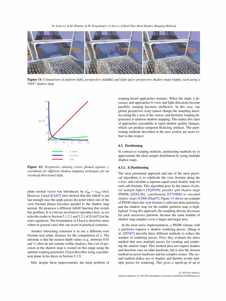
Figure 11: Comparison of uniform (left), perspective (middle) and light space perspective shadow maps (right), each using a10242 shadow map.

dp/ds

100

80

60

40

20

1

z

100806040201

LiSPSM

Uniform

PSM

Figure 12: Perspective aliasing errors plotted against z-coordinate for different shadow mapping techniques for anoverhead directional light.

plane normal vector was introduced, by n′opt = nopt/sinγ.However, Lloyd [Llo07] later showed that this falloff is notfast enough once the angle passes the point where one of theview frustum planes becomes parallel to the shadow mapnormal. He proposes a different falloff function that avoidsthis problem. It is a bit too involved to reproduce here, so werefer the reader to Section 5.1.2.1 and 5.2.1 of [Llo07] for theexact equations. The formulation of Lloyd is therefore morerobust in general cases that can occur in practical scenarios.

Another interesting extension is to use a different viewfrustum near plane distance for the computation of n. Therationale is that the nearest depth values (e.g., between 0.01and 1) often do not contain visible shadows, but a lot of pre-cision in the shadow map is wasted on this range using theoptimal warping parameter. Lloyd describes using a pseudo-near plane in his thesis in Section 5.1.9.

Still, despite these improvements, the main problem of

warping-based approaches remains: When the angle γ de-creases and approaches 0 (view and light directions becomeparallel), warping becomes ineffective. In this case, oneglobal perspective warp cannot change the sampling densi-ties along the z-axis of the viewer, and therefore warping de-generates to uniform shadow mapping. This makes this classof approaches susceptible to rapid shadow quality changes,which can produce temporal flickering artifacts. The parti-tioning methods described in the next section are more ro-bust in this respect.

4.3. Partitioning

In contrast to warping methods, partitioning methods try toapproximate the ideal sample distribution by using multipleshadow maps.

4.3.1. Z-Partitioning

The most prominent approach and one of the most practi-cal algorithms is to subdivide the view frustum along thez-axis, and calculate a separate equal-sized shadow map foreach sub-frustum. This algorithm goes by the names of plu-ral sunlight buffers [TQJN99], parallel split shadow maps(PSSM) [ZSXL06], z-partitioning [LTYM06] or cascadedshadow maps (CSM) [Eng07]. Figure 13 shows an exampleof PSSM where the view frustum is split into three partitions,and the shadow map for the middle partition map is high-lighted. Using this approach, the sampling density decreasesfor each successive partition, because the same number ofshadow map samples cover a larger and larger area.

In the most naive implementation, a PSSM scheme withn partitions requires n shadow rendering passes. Zhang etal. [ZSN07] describe three different methods to reduce thenumber of rendering passes. First, they evaluate the naivemethod that uses multiple passes for creating and render-ing the shadow maps. This method does not require shadersand therefore runs on older hardware, but is also the slowestmethod on newer hardware and for complex scenes. The sec-ond method makes use of shaders and thereby avoids mul-tiple passes for rendering. This gives a speed-up of up to



Figure 13: PSSM: Left: The shadow map for the middle ofthree partitions of the view frustum (side view) is empha-sized. Right: The bounding volumes for the partitions areshown in 3D. Inlays show the shadow maps.

30% on GeForce 8800 and newer. The third method usesthe geometry shader or advanced instancing to also avoidthe multiply passes to create the shadow maps by replicatingeach triangle into each of the required shadow maps duringthe shadow rendering pass. Although the authors mentionthat this method further increases performance, no numeri-cal data is given in their article to confirm this statement.

The most important question for this method is where toposition the split planes. One way is to go back to the deriva-tion of the shadow map resampling error. Each sub-shadowmap could be interpreted as a big texel of a global shadowmap, so that z-partitioning becomes a discretization of anarbitrary warping function. We have shown before that theoptimal warping function is logarithmic, therefore the splitpositions Ci should be determined as [LTYM06]:

Ci = zn

(zfzn

) im

where m is the number of partitions. However, as opposedto global warping schemes, the effect of z-partitioning isnot limited to the axes of the shadow map, but even workswhen the light is directly behind the viewer (see Figure 14).This is the main advantage of z-partitioning over warpingapproaches, and the reason why z-partitioning is much morerobust in general configurations. Figure 14, shows on the leftthe nearest and farthest partition in a situation with the lightdirectly behind the viewer. The shadow map for the nearestpartition covers a much smaller area, and therefore the per-ceived resolution is higher, just as is the case for the viewerprojection. For instance, Tadamura et al. [TQJN99] and En-gel [Eng07] partition the frustum along the view vector intogeometrically increasing sub-volumes. Figure 15 shows a di-rect comparison of z-partitioning vs. warping in the case ofa light from behind.

[ZSXL06] note that the optimal partition scheme is of-ten not practical because it allocates most resolution nearthe near plane, which is rarely populated with objects.

Figure 14: PSSM even works for cases were warping fails:for instance when the light is coming from behind.

They therefore propose computing the split positions asa weighted average between the logarithmic scheme anda simple equidistant split plane distribution. An alterna-tive solution that better respects the theoretical propertiesof shadow map aliasing is to use a pseudo-near plane justas in warping. This approach is explained in Lloyd’s the-sis [Llo07] in Section 5.1.8.

[ZZB09] also discuss a number of practical issues relatedto z-partitioning, regarding flickering artifacts, shadow mapstorage strategies, split selection, computation of texture co-ordinates, and filtering across splits. An interesting observa-tion is that in some cases, a point belonging to one parti-tion should be shadowed using a shadow map generated fora different partition. This happens when the light is almostparallel to the view direction. In this case, the shadow mapsfor the partitions nearer the view point will provide betterresolution.

Figure 15: For cases were the light is coming from be-hind, warping (left) gives unsatisfactory results, while z-partitioning (right) provides superior results. The shadowmap used for each fragment is color coded.

Still, optimizing the placement and sizes of z-partitionsby hand can give superior results, especially if not the wholedepth range is covered with shadows. To avoid this manual



tweaking, Lauritzen [Lau10] presented a probabilistic exten-sion to cascaded shadow maps. The idea is to analyze theshadow sample distribution required by the current frame tofind tight light-space bounds for each partition. The mainlimitation of this approach is that the clustering approach re-quires the calculation of a depth histogram, which is onlyfeasible on the latest hardware.

4.3.2. Frustum Face Partitioning

Another alternative partitioning scheme is to use a sepa-rate shadow map for each face of the view frustum as pro-jected onto the shadow map plane, and use warping foreach shadow map separately. This can also be interpreted asputting a cube map around the post-perspective view frus-tum and applying a shadow map to each cube face [Koz04].Each frustum face can be further split to increase quality.

This scheme is especially important because it can beshown that it is optimal for LogPSM, i.e., the combination oflogarithmic and perspective shadow mapping introduced byLloyd et al. [LGQ∗08]. However, we will not elaborate thisscheme here because Lloyd et al. [LGMM07] also showedthat for practical situations, i.e., a large far plane to nearplane ratio and a low number of shadow maps, z-partitioning(optionally combined with warping) is superior to frustumpartitioning.

A split into different shadow map buffers involving acoarse scene analysis is described by Forsyth [For06]. Theidea is that shadow receivers can be partitioned into dif-ferent shadow maps according to their distance to the viewpoint. An optimized projection can be used for each of theseclusters, thereby only generating shadows were needed. Thisscheme can have advantages if shadows only occur sparselyin a scene, but for general settings (shadows everywhere) itis identical to z-partitioning (with the added overhead of thescene analysis).

4.3.3. Adaptive Partitioning

The advantage of the partitioning algorithms discussed so faris that they are very fast. On the other hand, they completelyignore surface orientation and therefore do not improve un-dersampling due to surfaces that are viewed almost edge-onby the light source, i.e., projection aliasing.

There are a number of algorithms that try to allo-cate samples in a more optimal way by analyzing thescene before creating the shadow map. This inevitably in-curs some overhead due to the analysis step, but leads tomuch better results in general cases. This often necessi-tates a frame buffer read-back, which used to be a verycostly step. Nevertheless, this cost has been reduced onrecent hardware, which makes these methods more andmore interesting for practical use. Prominent examples areadaptive shadow maps (ASM) [FFBG01, LSK∗05], reso-lution matched shadow maps (RSMS) [LSO07], queried

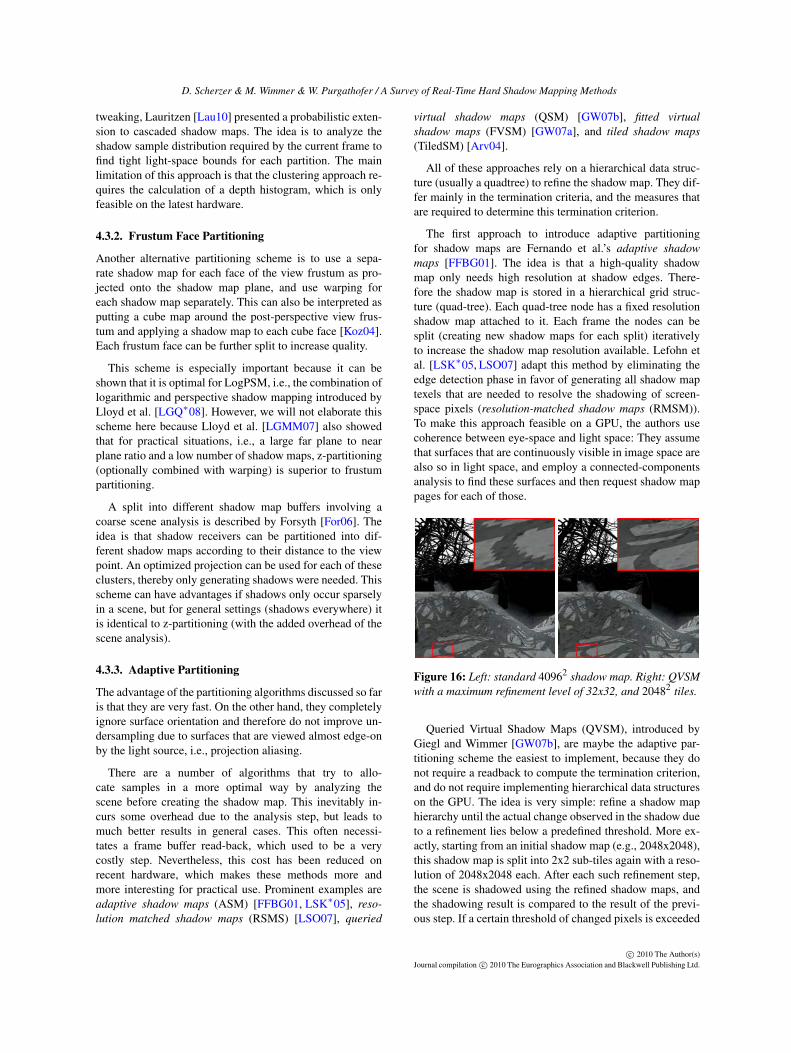
virtual shadow maps (QSM) [GW07b], fitted virtualshadow maps (FVSM) [GW07a], and tiled shadow maps(TiledSM) [Arv04].

All of these approaches rely on a hierarchical data struc-ture (usually a quadtree) to refine the shadow map. They dif-fer mainly in the termination criteria, and the measures thatare required to determine this termination criterion.

The first approach to introduce adaptive partitioningfor shadow maps are Fernando et al.’s adaptive shadowmaps [FFBG01]. The idea is that a high-quality shadowmap only needs high resolution at shadow edges. There-fore the shadow map is stored in a hierarchical grid struc-ture (quad-tree). Each quad-tree node has a fixed resolutionshadow map attached to it. Each frame the nodes can besplit (creating new shadow maps for each split) iterativelyto increase the shadow map resolution available. Lefohn etal. [LSK∗05, LSO07] adapt this method by eliminating theedge detection phase in favor of generating all shadow maptexels that are needed to resolve the shadowing of screen-space pixels (resolution-matched shadow maps (RMSM)).To make this approach feasible on a GPU, the authors usecoherence between eye-space and light space: They assumethat surfaces that are continuously visible in image space arealso so in light space, and employ a connected-componentsanalysis to find these surfaces and then request shadow mappages for each of those.

Figure 16: Left: standard 40962 shadow map. Right: QVSMwith a maximum refinement level of 32x32, and 20482 tiles.

Queried Virtual Shadow Maps (QVSM), introduced byGiegl and Wimmer [GW07b], are maybe the adaptive par-titioning scheme the easiest to implement, because they donot require a readback to compute the termination criterion,and do not require implementing hierarchical data structureson the GPU. The idea is very simple: refine a shadow maphierarchy until the actual change observed in the shadow dueto a refinement lies below a predefined threshold. More ex-actly, starting from an initial shadow map (e.g., 2048x2048),this shadow map is split into 2x2 sub-tiles again with a reso-lution of 2048x2048 each. After each such refinement step,the scene is shadowed using the refined shadow maps, andthe shadowing result is compared to the result of the previ-ous step. If a certain threshold of changed pixels is exceeded



in a tile, refinement continues. The way to make this fastis to do all calculations on the GPU by using the occlusionquery mechanism to count the number of pixels that differwhen applying a more refined shadow map in comparisonto the previous one. QVSM require a relatively high numberof scene rendering passes, one for each refinement attempt.In order to avoid re-rendering the scene multiple times, thescene is rendered into a linear depth-buffer first and each ren-dering pass just uses this buffer to calculate shadows (alsocalled deferred shadowing). Figure 16 shows a comparisonof a large standard shadow map with QVSM.

In order to avoid the high number of shadow renderingpasses in QVSMs, Giegl and Wimmer [GW07a] introducedFitted Virtual Shadow Maps (FVSM) to try to determine be-forehand what final refinement levels will be necessary in thequadtree. For this, the scene is rendered in a pre-pass, but in-stead of actually shadowing the scene, this pass just recordsthe query location into the shadow map, as well as the re-quired shadow map resolution at that query location. Theresulting buffer is then transferred to the CPU. There, eachsample of this buffer is transformed into shadow map spaceand stored in a low-resolution buffer, utilizing the efficientscattering capabilities of the CPU. This buffer ultimatelycontains the required resolution in each area of the shadowmap, and the quadtree structure can be derived from it. In or-der to reduce penalties due to readback, only a small frame-buffer (e.g., 256x256) is rendered in the pre-pass. In com-parison to Adaptive Shadow Maps [FFBG01,LSK∗05], bothQVSM and FVSM are fast enough to evaluate the whole hi-erarchy for each frame anew and therefore work well for dy-namic scenes, as opposed to ASM, which relies on an iter-ative edge-finding algorithm to determine refinement levels,and therefore needs to cache recently used tiles.

RMSM improve on ASMs especially for dynamic scenes,by avoiding the iterative step and calculating the requiredresolutions directly, somewhat similarly to FVSM. Both al-gorithms also mix data-parallel GPU algorithms [LKS∗06](like quadtree and sort) with standard rendering. In RMSMs,all steps are actually carried out on the GPU, while FVSMcompute the required subdivision levels on the CPU, but onlower resolution buffers.

Tiled shadow maps [Arv04] tile the light view (here afixed resolution shadow map) to change the sampling qual-ity according to a heuristical analysis based on depth dis-continuities, distances and other factors. This allows settinga hard memory limit, thereby trading speed against quality.

4.4. Comparison of Warping and Paritioning

Warping and partitioning are orthogonal approaches andcan therefore be combined. For instance, for z-partitioningeach partition can be rendered using LiSPSM. This in-creases quality especially for situations where LiSPSMworks well (overhead lights). Figure 17 shows the effect ofz-partitioning with and without warping.

Figure 17: Z-partitioning using 3 shadow maps with (left)and without (right) warping.

One special case of such a combination is to use one uni-form shadow map and one perspective shadow map and cal-culate a plane equation that separates areas where the one orthe other provides the best quality [Mik07].

Figure 18 shows the overall error (here called storage fac-tor), which takes into account error in both shadow mapdirections, of different schemes for different numbers ofshadow maps for overhead lights (ideal for warping) and alight behind (no warping possible).

Figure 18: Total error of different schemes for varyingshadow map numbers. FP is frustum face partitioning, ZPis z-partitioning, W is warping (figure courtesy of BrandonLloyd).

4.5. Irregular Sampling

In the second pass of shadow mapping, all screen-space frag-ments are reprojected into the shadow map to be queried.The aliasing artifacts in hard shadow mapping stem from thefact that the shadow map query locations do not correspondto the shadow map sample locations (see Figure 19). Ide-ally, one would like to create shadow map samples exactlyin those positions that will be queried later on. The idea ofirregular sampling methods is to render an initial eye spacepass to obtain the desired sample locations. These sample



locations are then used as pixel locations for the subsequentshadow map generation pass, thereby giving each screen-space fragment the best sample for the shadow map test andremoving all aliasing artifacts. The challenge is that thesenew sample locations do not lie on a regular grid anymore.Therefore, view sample accurate shadow algorithms have tosolve the problem of irregular rasterization.

Johnson at al. [JMB04, JLBM05] propose a hardware ex-tension: they store a list of reprojected view samples at eachregular shadow map grid element to allow for irregular sam-pling. They call this structure the irregular z-buffer. Withthis they can query the shadow test for each view sample byprojecting each shadow casting triangle from the viewpointof the light source. Each covered rasterized fragment has tobe tested against each of the stored view samples and thosein shadow are flagged. Unlike standard rasterization, whichonly creates a sample if the location at the center of a frag-ment is inside the rasterized polygon, this approach needsto calculate the overlap of each triangle with each fragment.This is necessary because the eye space samples are locatedat arbitrary positions inside each grid element. Finally, ascreen-space quad is rendered in eye-space, where each frag-ment does a shadow query by testing its corresponding listentry for the shadow flag.

Figure 19: Samples created on a regular grid in the shadowmap can be irregular in eye space (upper-left) and viceversa (upper-right). Therefore regular shadow mapping canlead to undersampling artifacts (lower-left) while irregularshadow mapping avoids artifacts by sampling the shadowmap for each eye space sample (lower-right).

Alias-free shadow maps [AL04] provide a hierarchicalsoftware implementation using an axis-aligned BSP tree toefficiently evaluate shadow information at the required sam-ple points. This approach was later mapped to graphics hard-ware by Arvo [Arv07] and Sintorn et al. [SEA08]. This ap-proach is very similar to Johnson et al.’s, but does not re-quire any hardware changes because the list stored at each

shadow map element is realized with a constant memoryfootprint. They are also able to map the overlap calculationto hardware by using conservative rasterization. The methodis suited to be combined with reparametrization methods andin practice, the authors implemented a variant of the fittingapproach described in [BAS02a]. Even accurate per-pixelshadows can be improved further by introducing supersam-pling. Pan et al. [PWC∗09] present such a method, whichavoids brute-force supersampling by extending [SEA08].The main idea is to approximate pixels by small 3d quad-rangles called facets (instead of just points). These facets al-low accounting for the area of a pixel. Potential blockers areprojected into screen-space via facets. Here occlusion maskswith multiple samples per pixel are used to calculate the sub-pixel shadows.

4.6. Temporal Reprojection

Finally, one way to increase the sampling rate is byreusing samples from previous frames through reprojec-tion [SJW07]. The main idea is to jitter the shadow mapviewport differently in each frame and to combine the re-sults over several frames, leading to a much higher effectiveresolution.

This method requires an additional buffer to store the ac-cumulated history of previous frames. In the current frame,the result of the shadow map lookup is combined with theaccumulated result calculated in the previous frames, whichcan be looked up using reprojection (to account for move-ment). If a depth discontinuity between the new and the re-projected sample is detected, then the old result is discardedsince it is probably due to a disocclusion.

Figure 20: LiSPSM gives good results for a shadow mapresolution of 10242 and a viewport of 1680×1050, but tem-poral reprojection can give even better results because it isnot limited by the shadow map resolution.

The shadow quality in this approach can actually be madeto converge to a pixel-perfect result by optimizing the choiceof the weight between the current and the previous frameresult (see Figure 20). The weight is determined accordingto the confidence of the shadow lookup:

confx,y = 1−max(|x− centerx| , |y− centery|

)·2,

where confx,y is the confidence for a fragment projected to



(x,y) in the shadow map and (centerx, centery) is the corre-sponding shadow map texel center.

The confidence is higher if the lookup falls near the centerof a shadow map texel, since only near the center of shadowmap texels it is very likely that the sample actually representsthe scene geometry.

Note that reprojection based approaches take a few framesto converge after quick motions. Also, they cannot deal verywell with moving objects or moving light sources. On theother hand, they practically eliminate temporal aliasing, forexample due to shadow map focusing.

5. Depth Biasing

A problem that is known by the name of incorrect self-shadowing or shadow acne is caused by undersamplingand the imprecision of the depth information stored in theshadow map for each texel. On the one hand, depth isrepresented with limited precision using either a fixed orfloating-point representation and these imprecisions can leadto wrong results. And on the other hand, the depth of each re-projected view space fragment is compared to a single depthfrom the shadow map. This depth is only correct at the orig-inal sampling point, but is used for the whole texel area. Ifthis texel area is big in view-space, due to undersampling, in-correct shadow test outputs can be the result (see Figure 21).

Figure 21: Left: A polygon is shadowing itself because ofinsufficient sampling and depth precision in the shadow map.Right: This results in z-fighting.

The standard solution is a user-defined depth bias, a smallincrement added to the shadow map depth values to movethem further away (see Figure 22, left). This moves theshadow caster away from the light and can therefore intro-duce light leaks if the new depth is farther away than thedepth of the receiver. This is most noticeable for contactshadows (see Figure 22, right). To make one bias setting ap-plicable to a wider range of geometry, most implementationsprovide a second parameter, which is dependent on the poly-gon slope (slope-scale biasing). Nevertheless, depth biasingis highly scene dependent and in general no automatic so-lution for an arbitrary scene exists. The main benefit of thismethod is its simplicity and support through hardware.

A factor that further aggravates the precision issues is thenon-linear distribution of depth values introduced by point(spot) lights, PSM, TSM, LispSM and similar reparameteri-zation methods. This non-linear distribution of depth valuesis generated by the perspective transformation that involvesa 1/w term, generating a hyperbolic depth value distribution.To counteract this, Brabec et al. [BAS02a] proposed linearlydistributed depth values. A similar approach was chosen fortrapezoidal shadow maps (TSM [MT04]), where the authorsrecommend omitting the z-coordinate from the perspectivetransformation. Kozlov [Koz04] proposes to use slope-scalebiasing for PSM in world-space and later transforms the re-sults into post-projective space. LispSM has less problemswith self-shadowing artifacts and can use normal slope-scalebiasing.

Figure 22: Depth biasing can remove incorrect self-shadowing (left), but can also introduce light leaks (right)if chosen too big.

To remove depth biasing, Woo [Woo92] proposed cal-culating the average of the first and second depth surfaceand consequently using this average depth (termed midpointshadow map) for the depth comparison. This introduces theoverhead of some form of depth peeling to acquire the sec-ond depth layer.

Second-depth shadow mapping, as proposed by Wang andMolnar [WM94], builds on the simple idea of using only thedepth of the second nearest surface to the light source, whichcan be done efficiently by backside rendering if shadowcasters are solid objects. The shadow map depth compari-son is therefore shifted to the back side of the casting ge-ometry, making the shadow test more robust for polygonsfacing the light source. In essence this introduces an adap-tive depth bias with the size of the thickness of the shadowcaster. This also introduces light leaks on shadow castingbacksides. Fortunately, these backsides can be determinedto be in shadow anyway by application of a standard diffuseillumination model. Nevertheless, due to possible huge dif-ferences in nearest and second nearest surface (huge shadowcaster thickness), imprecisions can arise. This problem is ad-dressed by Weiskopf and Ertl in dual shadow maps [WE03].They reintroduce a parameter that in effect limits the shadowcaster thickness.



A method that can avoid the need for biasing altogetherwas introduced by Hourcade and Nicolas [HN85]: a uniquepolygon id is stored instead of the depth in the shadow map.On comparison, either the same id is found (lit) or differentids are present (in shadow). To store the unique id, one 8bitchannel (256 ids) will be insufficient in most cases. Becauseonly one id can be stored per texel, the mechanism breaksdown if more than one triangle is present per texel.

6. Strategies to Reduce Reconstruction andOversampling Errors

The standard shadow map test results are binary: Either afragment is in shadow or not, creating hard jagged shadowmap edges for undersampled portions of the shadow map.From a signal processing point of view this correspondsto reconstruction using a box filter. Traditional bilinear re-construction as used for color textures is inappropriate forshadow maps, because a depth comparison to an interpolateddepth value still gives a (even more incorrect) binary resultinstead of an improved reconstruction.

Figure 23: Undersampled unfiltered shadow maps on theleft suffer from hard jagged edges. These can be removedby filtering. On the right hardware PCF with a 2x2 kernel isapplied.

Reeves et al. [RSC87] discovered that it makes muchmore sense to reconstruct the shadow test results and not theoriginal depth values. His percentage closer filtering (PCF)technique averages the results of multiple depth comparisonsin a Poisson disk sampling pattern in the shadow map to ob-tain in essence a (higher order) reconstruction filter for mag-nification of the shadow map. The smoothness of the result-ing shadow is directly related to the filter kernel size. Notethat this kernel has to be evaluated for each view space frag-ment, making the algorithm’s performance highly sensitiveto the kernel size. A faster variation of this method, alreadyimplemented directly in the texture samplers of current hard-ware, is to bilinearly filter the shadow map test results of thefour neighboring shadow map samples (see Figure 23).

Aliasing due to oversampling is usually avoided in imageprocessing by band-limiting the reconstructed signal beforeresampling it at the final pixel locations. For texture map-ping, prefiltering approaches such as mip-mapping are most

common. However, this is much harder to do for shadowmapping since the shadow function is not a linear transfor-mation of the depth map, and therefore the bandlimiting stepcannot be done before rendering. One option is to resort toon-the-fly filtering and evaluate PCF with large filter kernels,however this is slow and does not scale. Recent research pro-posed clever ways to reformulate the shadow test into a lin-ear function so that prefiltering can be applied.

One such reformulation are variance shadowmaps [DL06, Lau07] introduced by Donnelly and Lau-ritzen. They estimate the outcome of the depth test fora given PCF kernel by using mean and variance of thedepth value distribution inside this kernel window. Theadvantage is that mean and variance can be precomputedusing for example mip-mapping. The problem with thisapproach is that high variance in the depth distributions(high depth complexity) can lead to light leak artifacts (seeFigure 24, left) and high-precision (32 bit floating point)texture filtering hardware is needed for satisfying results. Asolution to both problems (layered variance shadow maps)was presented by Lauritzen and McCool [LM08], whopartition the depth range of the shadow map into multiplelayers. Although texture precision can be reduced withthis approach (even down to 8 bit), multiple layers are stillrequired for low variance.

Figure 24: Variance shadow maps (left), in contrast to con-volution shadow maps, suffer (right) from light leaks.

Another way to reformulate the binary shadow testwas introduced by Annen et al. with convolution shadowmaps [AMB∗07] (see Figure 24, right). Here instead of sta-tistical estimate, a Fourier expansion is used to representthe depth test. For a practical approximation using 16 co-efficients (from the infinitely many), 16 sine and 16 cosinetextures have to be stored. The expansion into a Fourier basisis a linear operation, so that prefiltering using mip-mappingof the individual basis textures can be applied. While the ba-sis textures require only 8 bit per texel (in comparison to24 bit for standard shadow maps), memory considerationsstill require a restriction of the Fourier expansion to a small



number of terms, which introduces ringing artifacts (Gibb’sphenomenon), again resulting in light leaks.

Following the same general idea, Annen et al. [AMS∗08]proposed exponential shadow maps, which replace theFourier expansion by an exponential. The idea is to interpretthe shadow test as a step function and use the exponential asa separable approximation of this step function. Here a sin-gle 32 bit texture channel is sufficient, making this approachmuch more memory friendly, but for larger kernel sizes thisapproximation does not hold anymore, leading to artifacts.

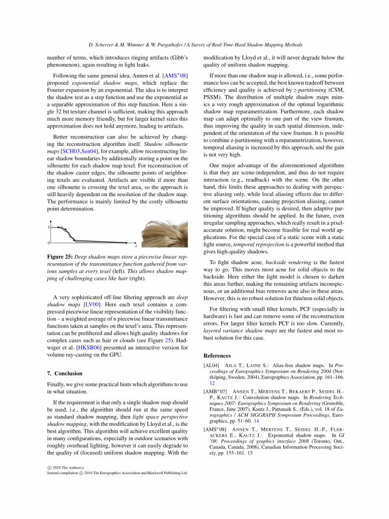
Better reconstruction can also be achieved by chang-ing the reconstruction algorithm itself. Shadow silhouettemaps [SCH03,Sen04], for example, allow reconstructing lin-ear shadow boundaries by additionally storing a point on thesilhouette for each shadow map texel. For reconstruction ofthe shadow caster edges, the silhouette points of neighbor-ing texels are evaluated. Artifacts are visible if more thanone silhouette is crossing the texel area, so the approach isstill heavily dependent on the resolution of the shadow map.The performance is mainly limited by the costly silhouettepoint determination.

z

1

0

Figure 25: Deep shadow maps store a piecewise linear rep-resentation of the transmittance function gathered from var-ious samples at every texel (left). This allows shadow map-ping of challenging cases like hair (right).

A very sophisticated off-line filtering approach are deepshadow maps [LV00]. Here each texel contains a com-pressed piecewise linear representation of the visibility func-tion – a weighted average of n piecewise linear transmittancefunctions taken at samples on the texel’s area. This represen-tation can be prefiltered and allows high quality shadows forcomplex cases such as hair or clouds (see Figure 25). Had-wiger et al. [HKSB06] presented an interactive version forvolume ray-casting on the GPU.

7. Conclusion

Finally, we give some practical hints which algorithms to usein what situation.

If the requirement is that only a single shadow map shouldbe used, i.e., the algorithm should run at the same speedas standard shadow mapping, then light space perspectiveshadow mapping, with the modification by Lloyd et al., is thebest algorithm. This algorithm will achieve excellent qualityin many configurations, especially in outdoor scenarios withroughly overhead lighting, however it can easily degrade tothe quality of (focused) uniform shadow mapping. With the

modification by Lloyd et al., it will never degrade below thequality of uniform shadow mapping.

If more than one shadow map is allowed, i.e., some perfor-mance loss can be accepted, the best known tradeoff betweenefficiency and quality is achieved by z-partitioning (CSM,PSSM). The distribution of multiple shadow maps mim-ics a very rough approximation of the optimal logarithmicshadow map reparametrization. Furthermore, each shadowmap can adapt optimally to one part of the view frustum,thus improving the quality in each spatial dimension, inde-pendent of the orientation of the view frustum. It is possibleto combine z-partitioning with a reparametrization, however,temporal aliasing is increased by this approach, and the gainis not very high.

One major advantage of the aforementioned algorithmsis that they are scene-independent, and thus do not requireinteraction (e.g., readback) with the scene. On the otherhand, this limits these approaches to dealing with perspec-tive aliasing only, while local aliasing effects due to differ-ent surface orientations, causing projection aliasing, cannotbe improved. If higher quality is desired, then adaptive par-titioning algorithms should be applied. In the future, evenirregular sampling approaches, which really result in a pixel-accurate solution, might become feasible for real world ap-plications. For the special case of a static scene with a staticlight source, temporal reprojection is a powerful method thatgives high-quality shadows.

To fight shadow acne, backside rendering is the fastestway to go. This moves most acne for solid objects to thebackside. Here either the light model is chosen to darkenthis areas further, making the remaining artifacts inconspic-uous, or an additional bias removes acne also in these areas.However, this is no robust solution for thin/non solid objects.

For filtering with small filter kernels, PCF (especially inhardware) is fast and can remove some of the reconstructionerrors. For larger filter kernels PCF is too slow. Currently,layered variance shadow maps are the fastest and most ro-bust solution for this case.

References[AL04] AILA T., LAINE S.: Alias-free shadow maps. In Pro-

ceedings of Eurographics Symposium on Rendering 2004 (Nor-rköping, Sweden, 2004), Eurographics Association, pp. 161–166.12

[AMB∗07] ANNEN T., MERTENS T., BEKAERT P., SEIDEL H.-P., KAUTZ J.: Convolution shadow maps. In Rendering Tech-niques 2007: Eurographics Symposium on Rendering (Grenoble,France, June 2007), Kautz J., Pattanaik S., (Eds.), vol. 18 of Eu-rographics / ACM SIGGRAPH Symposium Proceedings, Euro-graphics, pp. 51–60. 14

[AMS∗08] ANNEN T., MERTENS T., SEIDEL H.-P., FLER-ACKERS E., KAUTZ J.: Exponential shadow maps. In GI’08: Proceedings of graphics interface 2008 (Toronto, Ont.,Canada, Canada, 2008), Canadian Information Processing Soci-ety, pp. 155–161. 15



[Arv04] ARVO J.: Tiled shadow maps. In CGI ’04: Proceedingsof the Computer Graphics International (CGI’04) (Washington,DC, USA, 2004), IEEE Computer Society, pp. 240–247. 10, 11

[Arv07] ARVO J.: Alias-free shadow maps using graphics hard-ware. Journal of graphics, gpu, and game tools 12, 1 (2007),47–59. 12

[BAS02a] BRABEC S., ANNEN T., SEIDEL H.-P.: Practicalshadow mapping. Journal of Graphics Tools: JGT 7, 4 (2002),9–18. 5, 12, 13

[BAS02b] BRABEC S., ANNEN T., SEIDEL H.-P.: Shadow map-ping for hemispherical and omnidirectional light sources. InAdvances in Modelling, Animation and Rendering (ProceedingsComputer Graphics International 2002) (Bradford, UK, 2002),Vince J., Earnshaw R., (Eds.), Springer, pp. 397–408. 2

[CG04] CHONG H., GORTLER S. J.: A lixel for every pixel.In Proceedings of Eurographics Symposium on Rendering 2004(Norrköping, Sweden, 2004). 6

[CG07] CHONG H. Y., GORTLER S. J.: Scene Optimized ShadowMapping. Harvard Computer Science Technical Report: TR-07-07. Tech. rep., Harvard University, Cambridge, MA, 2007. 6

[Cho03] CHONG H.: Real-Time Perspective Optimal ShadowMaps. Senior thesis, Harvard College, Cambridge, Mas-sachusetts, Apr. 2003. 6

[Cro77] CROW F. C.: Shadow algorithms for computer graphics.In Proceedings of the 4th annual conference on Computer graph-ics and interactive techniques (New York, NY, USA, July 1977),George J., (Ed.), vol. 11, ACM Press, pp. 242–248. 2

[DL06] DONNELLY W., LAURITZEN A.: Variance shadow maps.In I3D ’06: Proceedings of the 2006 symposium on Interactive3D graphics and games (New York, NY, USA, 2006), ACM,pp. 161–165. 14

[Eng07] ENGEL W.: Cascaded shadow maps. In ShaderX5: Ad-vanced Rendering Techniques. Charles River Media, Inc., 2007.8, 9

[FFBG01] FERNANDO R., FERNANDEZ S., BALA K., GREEN-BERG D. P.: Adaptive shadow maps. In SIGGRAPH 2001 Con-ference Proceedings (Los Angeles, USA, Aug. 2001), Fiume E.,(Ed.), Annual Conference Series, ACM SIGGRAPH, AddisonWesley, pp. 387–390. 10, 11

[For06] FORSYTH T.: Making shadow buffers robust using multi-ple dynamic Shadow Maps. Charles River Media, 2006. 10

[GHFP08] GASCUEL J.-D., HOLZSCHUCH N., FOURNIER G.,PÉROCHE B.: Fast non-linear projections using graphics hard-ware. In I3D ’08: Proceedings of the 2008 symposium on Inter-active 3D graphics and games (Redwood City, California, 2008),ACM, pp. 107–114. 2

[GW07a] GIEGL M., WIMMER M.: Fitted virtual shadow maps.In Proceedings of GI (Graphics Interface) (Montreal, Canada,May 2007), Healey C. G., Lank E., (Eds.), Canadian Human-Computer Communications Society, pp. 159–168. 10, 11

[GW07b] GIEGL M., WIMMER M.: Queried virtual shadowmaps. In Proceedings of I3D (ACM SIGGRAPH Symposium onInteractive 3D Graphics and Games) (Seattle, WA, Apr. 2007),ACM Press, pp. 65–72. 10

[HKSB06] HADWIGER M., KRATZ A., SIGG C., BÜHLERK.: Gpu-accelerated deep shadow maps for direct volumerendering. In GH ’06: Proceedings of the 21st ACM SIG-GRAPH/EUROGRAPHICS symposium on Graphics hardware(New York, NY, USA, 2006), ACM, pp. 49–52. 15

[HLHS03] HASENFRATZ J.-M., LAPIERRE M., HOLZSCHUCHN., SILLION F.: A survey of real-time soft shadows algorithms.Computer Graphics Forum 22, 4 (dec 2003), 753–774. 1

[HN85] HOURCADE J. C., NICOLAS A.: Algorithms for an-tialiased cast shadows. Computers and Graphics 9, 3 (1985),259–265. 14

[JLBM05] JOHNSON G. S., LEE J., BURNS C. A., MARKW. R.: The irregular z-buffer: Hardware acceleration for irregu-lar data structures. ACM Trans. Graph. 24, 4 (2005), 1462–1482.12

[JMB04] JOHNSON G. S., MARK W. R., BURNS C. A.: TheIrregular Z-Buffer and its Application to Shadow Mapping. Re-search paper, The University of Texas at Austin, 2004. 12

[Koz04] KOZLOV S.: Perspective shadow maps - care and feed-ing. GPU Gems 1 (2004), 217–244. 10, 13

[Lau07] LAURITZEN A.: GPU Gems 3. Addison-Wesley, 2007,ch. Summed-Area Variance Shadow Maps. 14

[Lau10] LAURITZEN A.: Sample distribution shadow maps. InAdvances in Real-Time Rendering in 3D Graphics and Games(2010), SIGGRAPH Courses. 10

[LGMM07] LLOYD D. B., GOVINDARAJU N. K., MOLNARS. E., MANOCHA D.: Practical logarithmic rasterization forlow-error shadow maps. In Proceedings of Graphics Hard-ware (ACM SIGGRAPH/Eurographics Workshop on GH) (Aire-la-Ville, Switzerland, Switzerland, 2007), Eurographics Associa-tion, pp. 17–24. 7, 10

[LGQ∗08] LLOYD D. B., GOVINDARAJU N. K., QUAMMENC., MOLNAR S. E., MANOCHA D.: Logarithmic perspectiveshadow maps. ACM Transactions on Graphics 27, 4 (Oct. 2008),1–32. 4, 7, 10

[LKS∗06] LEFOHN A., KNISS J. M., STRZODKA R., SEN-GUPTA S., OWENS J. D.: Glift: Generic, efficient, random-access GPU data structures. ACM Transactions on Graphics 25,1 (Jan. 2006), 60–99. 11

[Llo07] LLOYD B.: Logarithmic Perspective Shadow Maps. PhDthesis, University of North Carolina at Chapel Hill, August 2007.4, 7, 8, 9

[LM08] LAURITZEN A., MCCOOL M.: Layered varianceshadow maps. In GI ’08: Proceedings of graphics interface 2008(Toronto, Ont., Canada, Canada, 2008), Canadian InformationProcessing Society, pp. 139–146. 14

[LSK∗05] LEFOHN A., SENGUPTA S., KNISS J. M., STR-ZODKA R., OWENS J. D.: Dynamic adaptive shadow maps ongraphics hardware. In ACM SIGGRAPH Conference Abstractsand Applications (Los Angeles, CA, Aug. 2005). 10, 11

[LSO07] LEFOHN A. E., SENGUPTA S., OWENS J. D.: Resolu-tion matched shadow maps. ACM Transactions on Graphics 26,4 (Oct. 2007), 20:1–20:17. 10

[LTYM06] LLOYD B., TUFT D., YOON S., MANOCHA D.:Warping and partitioning for low error shadow maps. In Proceed-ings of the Eurographics Symposium on Rendering 2006 (2006),Eurographics Association, pp. 215–226. 6, 8, 9

[LV00] LOKOVIC T., VEACH E.: Deep shadow maps. In Pro-ceedings of the 27th annual conference on Computer graphicsand interactive techniques (2000), ACM Press/Addison-WesleyPublishing Co., pp. 385–392. 15

[MBW08] MATTAUSCH O., BITTNER J., WIMMER M.: Chc++:Coherent hierarchical culling revisited. Computer Graphics Fo-rum (Proceedings Eurographics 2008) 27, 2 (Apr. 2008), 221–230. 5

[Mik07] MIKKELSEN M. S.: Separating-plane perspectiveshadow mapping. journal of graphics, gpu, and game tools 12, 3(2007), 43–54. 11



[MT04] MARTIN T., TAN T.-S.: Anti-aliasing and continuitywith trapezoidal shadow maps. In Proceedings of Eurograph-ics Symposium on Rendering 2004 (Norrköping, Sweden, 2004),pp. 153–160. 6, 13

[PWC∗09] PAN M., WANG R., CHEN W., ZHOU K., BAO H.:Fast, sub-pixel antialiased shadow maps. Computer Graphics Fo-rum 28, 7 (Oct. 2009), 1927–1934. 12

[RSC87] REEVES W. T., SALESIN D. H., COOK R. L.: Render-ing antialiased shadows with depth maps. In Computer Graphics(SIGGRAPH ’87 Proceedings) (July 1987), Stone M. C., (Ed.),vol. 21, pp. 283–291. 14

[SCH03] SEN P., CAMMARANO M., HANRAHAN P.: Shadowsilhouette maps. ACM Transactions on Graphics (Proceedingsof SIGGRAPH) 22, 3 (2003), 521–526. 15

[SD02] STAMMINGER M., DRETTAKIS G.: Perspective shadowmaps. In ACM Transactions on Graphics (Proceedings of SIG-GRAPH) (San Antonio, Texas, July 2002), ACM Press, pp. 557–562. 3, 4, 6

[SEA08] SINTORN E., EISEMANN E., ASSARSSON U.: Sample-based visibility for soft shadows using alias-free shadow maps.Computer Graphics Forum (Proceedings of the EurographicsSymposium on Rendering 2008) 27, 4 (June 2008), 1285–1292.12

[Sen04] SEN P.: Silhouette maps for improved texture magni-fication. In Proceedings of Graphics Hardware (ACM SIG-GRAPH/Eurographics Workshop on GH) (Grenoble, France,2004), ACM, pp. 65–73. 15

[SJW07] SCHERZER D., JESCHKE S., WIMMER M.: Pixel-correct shadow maps with temporal reprojection and shadow testconfidence. In Rendering Techniques 2007 (Proceedings Eu-rographics Symposium on Rendering) (Grenoble, France, June2007), Kautz J., Pattanaik S., (Eds.), Eurographics, EurographicsAssociation, pp. 45–50. 12

[TQJN99] TADAMURA K., QIN X., JIAO G., NAKAMAE E.:Rendering optimal solar shadows using plural sunlight depthbuffers. In CGI ’99: Proceedings of the International Conferenceon Computer Graphics (Washington, DC, USA, 1999), IEEEComputer Society, p. 166. 8, 9

[WE03] WEISKOPF D., ERTL T.: Shadow Mapping Based onDual Depth Layers. In Procceedings of Eurographics ’03 ShortPapers (Granada, Spain, 2003), pp. 53–60. 13

[Wil78] WILLIAMS L.: Casting curved shadows on curved sur-faces. Computer Graphics (SIGGRAPH ’78 Proceedings) 12, 3(Aug. 1978), 270–274. 2

[WM94] WANG Y., MOLNAR S.: Second-Depth Shadow Map-ping. Tech. rep., University of North Carolina at Chapel Hill,1994. 13

[Woo92] WOO A.: The shadow depth map revisited. GraphicsGems III (1992), 338–342. 13

[WPF90] WOO A., POULIN P., FOURNIER A.: A survey ofshadow algorithms. IEEE Computer Graphics and Applications10, 6 (Nov. 1990), 13–32. 1

[WS06] WIMMER M., SCHERZER D.: Robust shadow map-ping with light space perspective shadow maps. In ShaderX 4– Advanced Rendering Techniques, Engel W., (Ed.), vol. 4 ofShaderX. Charles River Media, Mar. 2006. 5

[WSP04] WIMMER M., SCHERZER D., PURGATHOFER W.:Light space perspective shadow maps. In Rendering Techniques(Proceedings of the Eurographics Symposium on Rendering)(Norrköping, Sweden, 2004), Springer Computer Science, Eu-rographics, Eurographics Association. 5, 6, 7

[ZSN07] ZHANG F., SUN H., NYMAN O.: Parallel-split shadowmaps on programmable gpus. In GPU Gems 3, Nguyen H., (Ed.).Addison-Wesley, Aug. 2007. 8

[ZSXL06] ZHANG F., SUN H., XU L., LUN L. K.: Parallel-splitshadow maps for large-scale virtual environments. In Proceed-ings of the 2006 ACM international conference on Virtual realitycontinuum and its applications (Hong Kong, China, 2006), VR-CIA ’06, ACM, pp. 311–318. 8, 9

[ZXTS06] ZHANG F., XU L., TAO C., SUN H.: Generalizedlinear perspective shadow map reparameterization. In Proceed-ings of VRCIA (International Conference on Virtual Reality Con-tinuum and Its Applications) (Hong Kong, China, 2006), ACM,pp. 339–342. 7

[ZZB09] ZHANG F., ZAPRIJAGAEV A., BENTHAM A.: Practicalcascaded shadow maps. In ShaderX 7 – Advanced RenderingTechniques, Engel W., (Ed.), vol. 7 of ShaderX. Charles RiverMedia, Mar. 2009. 6, 9


A Survey of Real-Time Hard Shadow Mapping Methods

Documents

Transcript of A Survey of Real-Time Hard Shadow Mapping Methods