A-study-on-framework-and-realizing-mechanism-of-ISEE ...

Journal of Software ISSN 1796-217X Volume 5, Number 10, October 2010 Contents Special Issue: Information Security and Applications

Guest Editor: Feng Gao, Bin Wang, Deyun Yang, Junhu Zhang, and Shifei Ding Guest Editorial Feng Gao, Bin Wang, Deyun Yang, Junhu Zhang, and Shifei Ding

1049

SPECIAL ISSUE PAPERS An Efficient XML Index for Keyword Query with Semantic Path in Database Yanzhong Jin and Xiaoyuan Bao Realtime and Embedded System Testing for Biomedical Applications Jinhe Wang, Jing Zhao, and Bing Yan Color Map and Polynomial Coefficient Map Mapping Huijian Huan and Caiming Zhang A Study on the Framework and Realizing Mechanism of ISEE Based on Product Line Jianli Dong and Ningguo Shi Cross-platform Transplant of Embedded Smart Devices Jing Zhang and XinGuan Li A Metrics Method for Software Architecture Adaptability Hong Yang, Rong Chen, and Ya-qin Liu ARM Static Library Identification Framework Qing Yin, Fei Huang, and Liehui Jiang Solving Flexible Multi-objective JSP Problem Using A Improved Genetic Algorithm Meng Lan, Ting-rong Xu, and Ling Peng Design and Implementation of Safety Expert Information Management System of Coal Mine Based on Fault Tree Cheng-gang Wang and Zi-zhen Wang A New Community Division based on Coring Graph Clustering Ling Peng, Ting-rong Xu, and Meng Lan

1052

1060

1068

1077

1084

1091

1099

1107

1114

1121

REGULAR PAPERS Multiprocessor Scheduling by Simulated Evolution Imtiaz Ahmad, Muhammad K. Dhodhi, and Ishfaq Ahmad

1128

The Chinese Text Categorization System with Category Priorities Huan-Chao Keh, Ding-An Chiang, Chih-Cheng Hsu, and Hui-Hua Huang A Pre-Injection Analysis for Identifying Fault-Injection Tests for Protocol Validation Neeraj Suri and Purnendu Sinha The Use of AHP in Security Policy Decision Making: An Open Office Calc Application Irfan Syamsuddin and Junseok Hwang Adaptive Multi-agent System: Cooperation and Structures Emergence Imane Boussebough, Ramdane Maamri, Zaïdi Sahnoun

1137

1144

1162

1170

Special Issue on Information Security and Applications

Guest Editorial

This special issue is partly associated with the 2009 International Work Shop on Information Security and Applications (IWISA 2009), which was held in Qingdao, China in November 2009.While some other manuscripts are solicited from the authors who are not participants of the conference. The purpose of this special issue is to provide a fast publication of extended versions of the high-quality conference papers on software or related to software and also the papers from authors with original high-quality contributions that have neither been published in nor submitted to any journals or refereed conferences. Papers are mainly interdisciplinary research in software related theory and software related techniques to unsolved problems, such as database management, Software Strategy, and embedded software development etc.

We received 21 papers from around the world and selected 10 to be included in the special issue after a thorough and rigorous review process. The presented papers are mainly devoted to discussion on software architecture and software strategy.

In “An Efficient XML Index for Keyword Query with Semantic Path in Database”, Yanzhong Jin et al proposes an XML index structure BTP-Index, composed of XML structure index mechanism which backbone is a Suffix tree, for evaluation of path ([//|/]e1[//|/]e2[//|/]…[//|/]em) of Q, and XML content index mechanism which is based on Tries & Patricia tree, for the evaluation of [text()=str], filtering part of query Q. Using BTP-Index, the author can process query Q efficiently. And the author has proven the effectiveness of BTP index in Relation-XML dual engine database management system..

In “Realtime & Embedded System Testing for Biomedical Applications”, Jinhe Wang,, et al, propose a software testing approach to build a testing architecture for biomedical applications , it can check the reliability based on the failure data observed during software testing and can be applied to make the use of test task more flexible. The reliability of data of the system is computed through the test panel and simulation of the testing system by testing the reliabilities of the individual modules in the embedded system.

In “Color Map and Polynomial Coefficient Map Mapping”, Huijian Han et al proposes an image-based method to fit the reflection mode by a quadratic multinomial. The coefficients of quadratic multinomial will be gained from BTFs and are stored for every texel as polynomial coefficient maps. A picture is taken under well-proportioned environment light as a color map, which the chromaticity is saved. The method can interpolate light effective under varying virtual lighting conditions by color map and coefficient maps and represent the variation of luminance and color for each text independently.

In “A Study on the Framework and Realizing Mechanism of ISEE Based on Product Line”, Jianli Dong et al put forward a new model of integrated software engineering environment based on product line and by using product line automatic production procedure and the management system of modern manufacturing industry for reference, and also the framework and realizing mechanism of the new model is analyzed.

In “Cross-platform Transplant of Embedded Smart Devices”, Jing Zhang et al present the procedures for intelligent devices were designed according to the features of Windows Embedded CE6.0 as well as the characteristics of Visual Studio.net 2005, and the build environment. FmodMp3 player program was designed with managed language and transplanted to different intelligent devices, then the goal of cross-platform transplantation, that “code once written then ran in different platform” is achieved. This paper also gave some advice on how to improve decompile capacity of managed programs.

In “A Metrics Method for Software Architecture Adaptability”, Hong Yang et al presents a new process-oriented metrics for software architecture adaptability based on GQM (Goal Question Metric) approach. This method extends and improves the GQM method. It develops process-oriented processes for metrics modeling, introduces data and validation levels, adds structured description of metrics, and defines new indexes of metrics.

In “ARM Static Library Identification Framework”, Yin Qing et al propose a static library identification framework through studying library as “dcc”, which dynamically extracts binary characteristic file on applications under ARM processor.

In “Solving Flexible Multi-objective JSP Problem Using A Improved Genetic Algorithm”, Meng Lan et al propose an improved genetic algorithm for multi-objective Flexible JSP (job shop scheduling) problem. The algorithm construct the initial solution based on judging similarity strategy and immune mechanisms, proposed a self-adaptation cross and mutation operator, and using simulated annealing algorithm strategy combined with immune mechanisms in the selection operator, the experiment proof shows that, the improved genetic algorithm can improve the performance.

In “Design and Implementation of Safety Expert Information Management System of Coal Mine Based on Fault Tree”, WANG Cheng-gang et al firstly introduce the overall structure and the component of the expert system, illustrate the fault tree analysis method in detail; then describe the key technologies and implementation method of software development and the program is given; finally, explain the important role of system implementation in solving the safety information management problem of coal mine.

JOURNAL OF SOFTWARE, VOL. 5, NO. 10, OCTOBER 2010 1049

© 2010 ACADEMY PUBLISHERdoi:10.4304/jsw.5.10.1049-1051

In “A New Community Division based on Coring Graph Clustering”, Peng Ling et al propose A new community finding algorithm, based on the greedy algorithm with graph clustering by computing the density variation sequence and identifying core nodes, number of communities, partition the certain nodes to some belonged community with the similarity of characteristics of communication behavior by continuous readjusting the centrality of the communities.

Hopefully, this Special Issue will contribute to enhancing knowledge in many diverse areas of the software and some software related area. The author wishes to extend his thanks to Dr. Xijun Zhu who have done a lot of work in soliciting papers to this special issue, and to all those who kindly participated as peer reviewers. Their involvement was greatly appreciated.

We also thank Mrs. George J. Sun, the Executive Editor-in-Chief of JNW for his continued encouragement, guidance and support in the preparation of this issue.

Guest Editors: Feng Gao, Qingdao Technological University, China Bin Wang, Qingdao Technological University, China Deyun Yang, Qingdao Technological University, China Junhu Zhang, Taishan University, China Shifei Ding, China University of Mining andTechnology, China

Feng Gao graduated from Dalian University of Technology in 2004 with a Ph.D. degree in numerical analysis. He currently is a Professor in the Faculty of Science School of Qingdao Technological University. He has more than 20 research publications, chaired International Conferences and Workshops, and served on the editorial committee of many journals. His current research interest is in approximation theory and its applications.

Bin Wang got his Ph.D. degree in Xian Jiaotong University and currently is a professor with Computer Science Engineering School of Qingdao Technological University. His current research area is trustworthy computing and information security.

Junhu Zhang received his PhD degree in computer science from Peking University, Beijing, China in 2006. He is currently an Assistant Professor of Computer Science at Qingdao Technological University, China. He was a Post-doctor at LIAMA (Sino-French Laboratory for computer Science, Automation and Applied Mathematics) in the institute of Automation, Chinese Academy of Science from 2006 to 2008. His current research interests are on ad-hoc networks, wireless sensor networks, data grids, distributed database systems, peer to-peer systems, embedded systems.

1050 JOURNAL OF SOFTWARE, VOL. 5, NO. 10, OCTOBER 2010

© 2010 ACADEMY PUBLISHER

Deyun Yang is a professor with information department of Taishan University.His research area is Data processing and Information Security. He is also the editor of the journal of IEEE Transactions on Signal Processing and Journal of Science in China。

Shifei Ding is a professor with China University of Mining &Technology. His current research interest is Computer science. He serves in many computer science research institutions, chaired many international conferences and he also is the editor of many international journals such as JIS, IFS and INS.



An Efficient XML Index for Keyword Query with Semantic Path in Database

Yanzhong Jin

Computer Science & Technology Department, Tianjin University of Science & Technology, Tianjin, China Email: [email protected]

Xiaoyuan Bao

Computer Science & Technology Department, Peking University, Beijing, China Tianjin Normal University, Tianjin, China

Email: [email protected]

Abstract—with the wide adoption of XML in many applications, people begin to manage thousands of XML documents in database. In many applications which backend data source powered by a XML database management system, keyword search is important to query XML data with a regular structure if the user does not know the structure or only knows the structure partially. Essentially, many keyword search can be rewritten to XPath query Q=[//|/]e1[//|/]e2[//|/]…[//|/]em[text()=str]-suppose there is a keyword search [books William] on XML data about publishing, the result could be the union of the results of the two queries after database system rewriting based on meta data: //books//chapters//authors[text()=”William”] and //books//authors[text()=”William”]. We propose an XML index structure BTP-Index, composed of XML structure index mechanism which backbone is a Suffix tree, for evaluation of path ([//|/]e1[//|/]e2[//|/]…[//|/]em) of Q, and XML content index mechanism which is based on Tries & Patricia tree, for the evaluation of [text()=str], filtering part of query Q. Using BTP-Index, we can process query Q efficiently. We have proven the effectiveness of BTP index in our Relation-XML dual engine database management system. Index Terms—XML, Suffix Tree, Index, XPath

I. INTRODUCTION

With the wide adoption of XML in many applications, people begin to manage thousands of XML documents in database. In many applications which backend data source powered by a XML database management system, keyword search with semantic constraint is important to query XML data with a regular structure if the user does not know the structure or only knows the structure partially. Essentially, many keywords search have the form Q=[//|/]e1[//|/]e2[//|/]…[//|/]em[text()=str] from the perspective of XPath[9]. For example, suppose there is a keyword search [books William] on XML data about publishing, the result could be the union of the results of the two queries after database system rewriting based on meta data: //books//chapters//authors[text()=”William”] and //books//authors[text()=”William”]. We focus this paper on index mechanism on which query Q will be evaluated efficiently in XML database. Query rewrites and optimization is beyond this paper.

As for query Q, it is to find all the elementm which has the text content str, and its ancestor/parent element is

elementm-1, which in turn has the ancestor/parent element elementm-2, and so on. In the following, we use notation Qs as the shortcut of the path [//|/]e1[//|/]e2[//|/]…[//|/]em of the query, and Qc for [text()=string], for simplicity.

As for the efficient query evaluation in database system, constructing indexes for the data over which query will be performed is a classical and effective idea. In database research and engineering fields, many XML indexes have been proposed over the last decade. Some representative index structure such as Structure Join based Index[1,2,3], Path based Index[4,5], APEX[6] and ViST[7], Graph Indexing[8], etc, have been proposed in recent years.

To our best knowledge, there is no solution for the evaluation of query Q, especially Qs at O(m) cost which m is the length of Qs.

A. Related works In structure join-based index [1], Quanzhong Li et al.

proposed a new system for indexing and storing XML data based on a numbering scheme for elements. This numbering scheme quickly determines the ancestor-descendant relationship between elements in the hierarchy of XML data. Reference [2] proposed a variation of the traditional merge join algorithm, called the multi-predicate merge join (MPMGJN) algorithm, for finding all occurrences of the basic structural relationships (such as containment queries). Similarly, ref. [3] developed two families of structure join algorithms tree-merge and stack-tree, for determination of ancestor-descendant relationships.

As for Path-based Index[4,5], DataGuides[4] is the structural summaries of the source XML data, and it can be used to find elements when their full path (path from root element) is given. But for some XML data, the index volume may be bigger than the source data. In ref. [5], BF. Cooper et al. proposed an Index Fabric, it is conceptually similar to the DataGuides in that it indexes all raw paths starting from the root element.

APEX[6] is an adaptive path index for XML data. Unlike the traditional techniques, APEX uses data mining algorithms to summarize paths that appear frequently in the query workload. It maintains every path of length two,



therefore it also has to rely on join operations to answer path queries with more than two elements.

ViST[7] has proposed a method for indexing XML data based on pre-sequencing XML data, so query evaluation is equivalent to the sequence matching.

Xifeng Yan et al. proposed in ref. [8] a graph mining technique, different from the existing path-based methods, a gIndex was proposed to make use of frequent substructures as the basic indexing feature.

Recently, ref. [15] considers indexing support for queries that combine keywords and structure, it described several extensions to inverted lists to capture structure when it is present.

As for keyword search in XML data, it is a hot database research topic in nowadays, ref. [16~25] are samples of these; ref. [16] proposed an extension to XML query languages that enables keyword search at the granularity of XML elements; ref. [17] considered the problem of efficiently producing ranked results for keyword search queries over hyperlinked XML documents, etc.

All these proposed index structures or methods cannot process Qs with keywords efficiently, and we don’t find practical methods which incorporating database management system can be used in our application example presented above, this motivates our work on BTP-index in a real database management system.

B. Related works For evaluating query Q efficiently, we propose an

XML index structure BTP-Index. In particular, the contributions of our paper can be described as follows:

We propose Suffix tree based XML structure index mechanism (B part of BTP-Index). Using this index mechanism, we can process the Basic Path Query Unit (see definition 1) of Q at time expense of O(h).

We propose an algorithm for processing Qs by join the Basic Path Query Unit result, based on an extended code mechanism for XML data tree.

We propose an XML content index structure based on Tries & Patricia[12] tree (TP part of BTP-Index). Each leaf node in the index tree corresponds to a word in XML content, and each item of the attached inverted list to the node contains position information of the word. And the worst evaluation cost of Qc is O(|str|+k* logB(|L|)). Put above structures together, we call the overval mechanism as BTP-Index.

We have implemented part of the methods in our Relation-XML dual engine DBMS system, and our experimental result perform in the system demonstrates the efficiency of BTP-Index.

The rest of this paper is organized as follows: Some related preliminary knowledge is introduced in section 2. In section 3, we propose the suffix based XML index mechanism and the algorithm joining Basic Path Query Unit efficiently, for evaluation of Qs. Section 4 proposes an XML content index structure for evaluation of Qc. In section 5, experimental results and brief analysis are given. Section 6 concludes the whole paper.

II. PRELIMINARIES

In this section, we introduce XPath and basic path query unit concept in II.A, then present the XML data model in II.B, and finally define Suffix tree and give some lemmas about it in II.C.

A. Basic Path Query Unit Definition 1. Basic Path Query Unit We call any XPath query of form //e1/e2/…/eh as a

Basic Path Query Unit of query Q.We will use BPQU as a shortcut for it.

Our overall idea to process structural part of query Q is to decompose the structural part of query Q into many BPQU, and processing each BPQU respectively first, then join the results of BPQU’s to get the final result of structural query part of Q.

Please note that the “structural part of query” has the same meaning with “semantic path of query” in our paper, we will use it interchangeable in the paper followed. Its notation Qs is also used in text sometimes.

B. XML data model We use a semi-structured data model called Object

Exchange Model[13] (OEM) to describe the content of XML document. A diagram is used to represent the data. In this diagram, nodes denote the objects and edges are tagged by attribute names. There are two kinds of OEM objects, Atomic object and Complex object. The value of Atomic object is undividable, ex. an integer, while the value of Complex object is a set of <label, id> pairs.

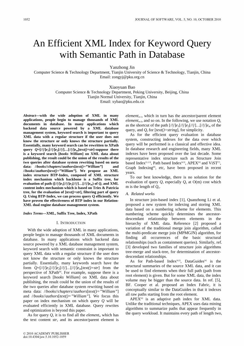
Fig. 1 a. Example of XML document b. OEM diagram

In OEM, XML data can be expressed as follows: OEM nodes denote XML elements and the relationship like parent-child, element-attribute and references are denoted by labeled edges. The data value (Suppose all the data values are string) corresponds to OEM leaves.

Fig. 1a shows the example of XML document in this paper and Fig. 1b is the corresponding OEM diagram. &0 and &1 are identifiers of elements. &13 and &14 are Atomic objects while &1 and &2 are Complex objects.

C. Suffix Tree Definition 2. String suffix Given a set ∑ of alphabet, s∈∑+∪ε; we call string

P is the suffix of S, iif(P=S[1,i], i=1,2,…,|S|, |S| is the length of S . Especially, empty string ε is also the suffix of S . In fact, ε is the suffix of any string.

Definition 3. String containment (⊆) Given two strings S1[1..m], S2[1..n] ∈∑+, m≤n.If

S1[1]= S2[i], S1[2]= S2[i+1],…, S1[m]= S2[i+m-



1],1≤i≤n-m+1, then we say that S1 contained in S2 (notation is S1⊆S2).

Definition 4. String suffix tree (TS) The suffix tree T of string S is a rooted tree. Formally,

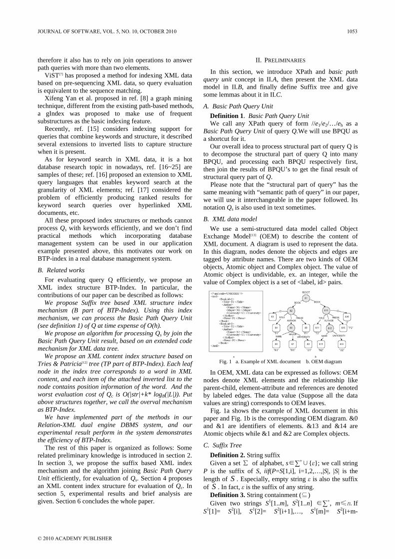
T=V,root,E,L,∑, among which, root is the root node; V is the set of all nodes in T; E is the set of all labeled edges in T; L is the set of all leaf nodes and L⊂V. ∀n∈V, there is a sequence l1l2...li, which we called the path of n. Actually, l1l2...li is the concatenation of edge labels along the path from root node to n. For each node n∈V, its path is unique. And for each leaf node m∈L, the edge path of m is one suffix of S. Fig. 2 is an example suffix tree of “ababc”.

Definition 5. Suffix tree containment Given T=V,root,E,T,∑ and T’=V’,root’,E’,T’, ∑’, if

V⊆V’∧E⊆E’∧ ∑⊆∑’, we say that T is contained in T’ (T⊆T’).

Based on the definitions above and suffix tree construction algorithm[11], we have the following propositions.

Lemma 1. The judgment of containment of string p in s can be implemented as the process of searching in suffix tree of s character by character from the root node, the time expense is o(m), where m is the length of p.

Lemma 2. Give string s1, s2, if s1⊆s2, we have Ts1⊆Ts2.

Fig. 2 Suffix tree of string “ababc”

III. XML STRUCTURE INDEX MECHANISM FOR EVALUATION OF BPQU

In this section, firstly we discuss the construction of XML structure index (B part of BTP-Index) for evaluation of basic path query unit in detail (III.A)(so we named it BPQU-Index), after that we analysis the query efficiency based on it (III.B) and (III.C) give the steps for evaluation of semantic path query of Q.

A. Index Construction Suppose there is an XML tree To(Vo,rooto,Eo,To,∑o)

(as Fig. 1b) where ∑o is the set of labels of all the edges of the tree. For Fig. 1, ∑o = book, title, author, name, major, university, press. Since all XML documents use “xml” as the root element, we don’t make it an element of ∑ o The path of nodes in To, for example, “book.author.name” of node “&6” and “book.author” of internal node “&5”, are path strings based on ∑o.

We found that node &4 and &11 are the same in semantics but different in contents. In order to represent the nodes of the same semantic, we define two kinds of path: data path and semantic path. Data path is a string of

format “l1d1l2d2…lidi”, where lk (k=1,2,…,i) is the tag of edge in OEM and dk (k=1,…,i) is the identifier of node, ex. &2 and &10. Semantic path is a string of format “l1l2…li”, where lk (k=1,2,…,i) is the tag of edge in OEM. Obviously a semantic path can have several data path. lk and dk are basic elements of the following algorithms like the single character of processing the string.

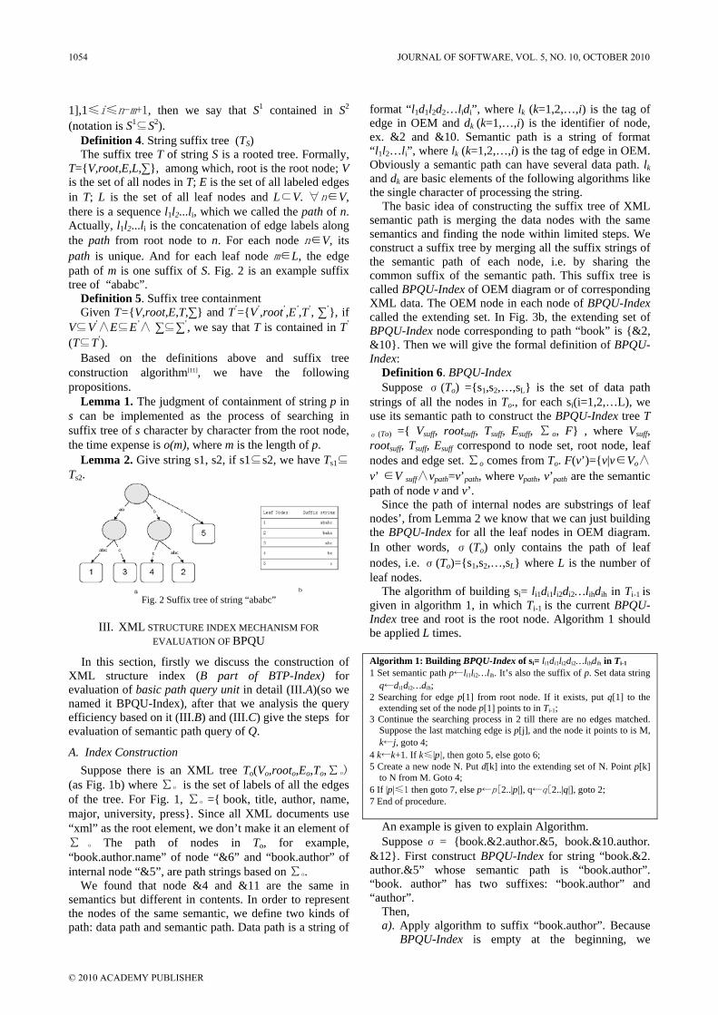
The basic idea of constructing the suffix tree of XML semantic path is merging the data nodes with the same semantics and finding the node within limited steps. We construct a suffix tree by merging all the suffix strings of the semantic path of each node, i.e. by sharing the common suffix of the semantic path. This suffix tree is called BPQU-Index of OEM diagram or of corresponding XML data. The OEM node in each node of BPQU-Index called the extending set. In Fig. 3b, the extending set of BPQU-Index node corresponding to path “book” is &2, &10. Then we will give the formal definition of BPQU-Index:

Definition 6. BPQU-Index Suppose σ(To) =s1,s2,…,sL is the set of data path

strings of all the nodes in To., for each si(i=1,2,…L), we use its semantic path to construct the BPQU-Index tree Tσ (To) = Vsuff, rootsuff, Tsuff, Esuff, ∑o, F , where Vsuff, rootsuff, Tsuff, Esuff correspond to node set, root node, leaf nodes and edge set. ∑o comes from To. F(v’)=v|v∈Vo∧

v’ ∈V suff∧vpath=v’path, where vpath, v’path are the semantic path of node v and v’.

Since the path of internal nodes are substrings of leaf nodes’, from Lemma 2 we know that we can just building the BPQU-Index for all the leaf nodes in OEM diagram. In other words, σ (To) only contains the path of leaf nodes, i.e. σ(To)=s1,s2,…,sL where L is the number of leaf nodes.

The algorithm of building si= li1di1li2di2…lihdih in Ti-1 is given in algorithm 1, in which Ti-1 is the current BPQU-Index tree and root is the root node. Algorithm 1 should be applied L times.

Algorithm 1: Building BPQU-Index of si= li1di1li2di2…lihdih in Ti-1 1 Set semantic path p←li1li2…lih. It’s also the suffix of p. Set data string

q←di1di2…dih; 2 Searching for edge p[1] from root node. If it exists, put q[1] to the

extending set of the node p[1] points to in Ti-1; 3 Continue the searching process in 2 till there are no edges matched.

Suppose the last matching edge is p[j], and the node it points to is M, k←j, goto 4;

4 k←k+1. If k≤|p|, then goto 5, else goto 6; 5 Create a new node N. Put d[k] into the extending set of N. Point p[k]

to N from M. Goto 4; 6 If |p|≤1 then goto 7, else p←p[2..|p|], q←q[2..|q|], goto 2; 7 End of procedure.

An example is given to explain Algorithm. Suppose σ = book.&2.author.&5, book.&10.author.

&12. First construct BPQU-Index for string “book.&2. author.&5” whose semantic path is “book.author”. “book. author” has two suffixes: “book.author” and “author”.

Then, a). Apply algorithm to suffix “book.author”. Because

BPQU-Index is empty at the beginning, we



construct root node first. Then create node “&2”, edge “book”, node “&5” and edge “author”;

b). Apply algorithm to suffix “author”. Because the root node doesn’t have an edge labeled “author”, we create edge “author” and node “&5”. Fig. 3a shows the resulting BPQU-Index. Then process “book.&10.author. &12” based on the BPQU-Index now;

c). Apply algorithm to suffix “book.author”. Edge “book” is found from the root node and it points to node “&2”. Merge “&10” into it and get &2,&10. Then edge “author” is found to match the following edge. Add “&12” into the node which “author” points to and get &5,&12;

d). Apply algorithm to suffix “book.author”. Similar to c), “&12” is merged into node which “author” points to and get &5,&12. The resulting BPQU-Index is shown in Fig. 3b.

In Fig. 1b, because most of the data path of node “&6” and “&7” are overlapped, if first adding the suffix of path of node “&6” as algorithm 1, the constructing of suffix of node “&7” contributes little to the extending set of the corresponding path. Actually, for leaf nodes in OEM diagram, if some of the data paths are overlapped, there will be some redundant work for algorithm 1. The time complexity of algorithm 1 is O(h2).

Fig 3. a. BPQU-Index of “book.&2.author.&5”

b.BPQU-Index after processing “book.&10.author.&12”

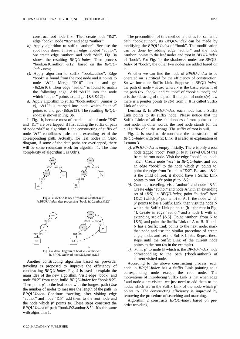
Fig. 4 a. data Diagram of book.&2.author.&5

b. BPQU-Index of book.&2.author.&5

Another constructing algorithm based on pre-order traveling is proposed to improve the efficiency of constructing BPQU-Index. Fig. 4 is used to explain the main idea of the new algorithm: Visit edge “book” and node “&2” from root, build BPQU-Index for “book.&2”. Then point p’ to the leaf node with the longest path (Use the number of nodes to measure the length of the path) in BPQU-Index. Continue traveling, after visiting edge “author” and node “&5”, add them to the root node and the node which p’ points to. These steps construct the BPQU-Index of path “book.&2.author.&5”. It’s the same with algorithm 1.

The precondition of this method is that as for semantic path “book.author”, its BPQU-Index can be made by modifying the BPQU-Index of “book”. The modification can be done by adding edge “author” and the node “author” points to the leaf nodes and root in BPQU-Index of “book”. For Fig. 4b, the shadowed nodes are BPQU-Index of “book”, the other two nodes are added based on it.

Whether we can find the node of BPQU-Index to be operated on is critical for the efficiency of construction. So we introduce Suffix Link. Suppose in BPQU-Index, the path of node v is xα, where x is the basic element of the path (ex. “book” and “author” of “book.author”) and α is the substring of the path. If the path of node s(v) is α there is a pointer points to s(v) from v. It is called Suffix Link of node v.

Lemma 3. In BPQU-Index, each node has a Suffix Link points to its suffix node. Please notice that the Suffix Links of all the child nodes of root point to the root node. In other words, the root node stands for the null suffix of all the strings. The suffix of root is null.

Fig. 4 is used to demonstrate the construction of BPQU-Index with Suffix Link. It is also an explanation of Lemma 3.

a). BPQU-Index is empty initially. There is only a root node tagged “root”. Point p’ to it. Travel OEM tree from the root node. Visit the edge “book” and node “&2”. Create node “&2” in BPQU-Index and add an edge “book” to the node which p’ points to, point the edge from “root” to “&2”. Because “&2” is the child of root, it should have a Suffix Link points to root. We point p’ to “&2”.

b). Continue traveling, visit “author” and node “&5”. Create edge “author” and node A with an extending set of &5 in BPQU-Index, point “author” from &2 (which p’ points to) to A. If the node which p’ points to has a Suffix Link, then visit the node N which the Suffix Link points to (It’s the root in Fig. 4). Create an edge “author” and a node B with an extending set of &5. Point “author” from N to &5 and point the Suffix Link of A to B. If node N has a Suffix Link points to the next node, mark that node and use the similar procedure of create edge, nodes and set the Suffix Links. Repeat these steps until the Suffix Link of the current node points to the root (as in the example).

c). Point p’ to node B which is the BPQU-Index node corresponding to the path (“book.author”) of current visited node.

According to the above constructing process, each node in BPQU-Index has a Suffix Link pointing to a corresponding node except the root node. The motivations of introducing Suffix Link is that when edge l and node n are visited, we just need to add them to the nodes which are in the Suffix Link of the node which p’ points to. The constructing efficiency is improved by removing the procedure of searching and matching.

Algorithm 2 constructs BPQU-Index based on pre-order traveling.



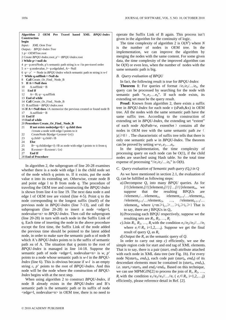
Algorithm 2 OEM Pre Travel based XML BPQU-Index Construction begin Input： XML Oem Tree Output： BPQU-Index Tree 1 p←OEMTree.root 2 Create BPQU-Index.root; p’←BPQU-Index.root 3 While p<>null do 4 p←p.nextNode, p’s semantic path string is w //in pre-travel order 5 n ←p.nodevalue, l←p.edgelabel, A←Null 6 q←p’←Node in BPQU-Index which semantic path m string is w-l 7 While q.sufflink<>Null do 8 Call Create_Or_Find_ Node_B 9 If A<>Null then 10 A.sufflink←B 11 End If 12 A←B; q←q.sufflink 13 End of while 14 Call Create_Or_Find_ Node_B 15 B.sufflink←BPQU-Index.root 16 If A<>Null then //A memorize the previous created or found node B 17 A.sufflink←B 18 End If 19 End of while 20 Procedure Create_Or_Find_ Node_B 21 If not exists node(edge=l) ∉ q.child then //create a node with edge l points to it 22 CreateNode B(edge=l,extent=n) 23 q.child←q.child∪B 24 Else 25 B←q.child(edge=l) //B as node with edge l points to it from q 26 B.extent←B.extent∪n 27 End If 28 End of Procedure

In algorithm 2, the subprogram of line 20-28 examines whether there is a node with edge l in the child node set of the node which q points to. If it exists, put the node value n into its extending set. Otherwise, create node B and point edge l to B from node q. The procedure of traveling the OEM tree and constructing the BPQU-Index is shown from line 4 to line 19. The next data node n and edge l of OEM tree are visited (line 4-5). Point q to the node corresponding to the longest suffix (itself) of the previous node in BPQU-Index (line 7-13), and call the subprogram (line 20-28) to insert a node <edge=l, nodevalue=n> to BPQU-Index. Then call the subprogram (line 20-28) in turn with each node in the Suffix Link of q. Each time of inserting the node in the above procedure except the first time, the Suffix Link of the node added the previous time should be pointed to the latest added node, in order to make sure the semantic path α of node B which A’s BPQU-Index points to is the suffix of semantic path xα of A. The situation that q points to the root of BPQU-Index is managed in line 14-18. Suppose the semantic path of node <edge=l, nodevalue=n> is w, p’ points to a node whose semantic path is w-l in the BPQU-Index (line 6). This is obvious because if w-l is an empty string ε, p’ points to the root of BPQU-Index. And this node will be the node where the construction of BPQU-Index begins with at the next step.

When using algorithm 2 to construct BPQU-Index, if node B already exists in the BPQU-Index and B’s semantic path is the semantic path or its suffix of node <edge=l, nodevalue=n> in OEM tree, there is no need to

operate the Suffix Link of B again. This process isn’t given in the algorithm for the continuity of logic.

The time complexity of algorithm 2 is O(N2) where N is the number of nodes in OEM tree. In the implementation, we can improve the algorithm by merging the nodes with the same content. For some given data, the time complexity of the improved algorithm can be O(N) or even less, when the number of nodes with the same semantic path is big.

B. Query evaluation of BPQU In fact, the following result is true for BPQU-Index: Theorem 1: For queries of format //e1/e2/…/eh, the

query can be processed by searching for the node with semantic path “e1.e2….eh”. If such node exists, its extending set must be the query result.

Proof: Known from algorithm 2, there exists a suffix tree in BPQU-Index for each node v (sPath,&x) in OEM tree. All the nodes with the same semantic path have the same suffix tree. According to the construction of extending set in BPQU-Index, the extending set “extent” of each node A(sPath=w, extentSet） contains all the nodes in OEM tree with the same semantic path zw（

|z|≥0）. The characteristic of suffix tree tells that there is only one semantic path w in BPQU-Index. The theorem can be proved by setting w=e1.e2….eh.

In the implementation, the time complexity of processing query on each node can be O(1), if the child nodes are searched using Hash table. So the total time expense of processing “//e1/e2/…/eh” is O(h).

C. Query evaluation of Semantic path query (Qs) in Q As we have mentioned in section 2.1, the evaluation of

Qs can be fulfilled as following steps: a).Decompose Qs into many BPQU queries. As for

[//|/]element1[//|/]element2[//|/]…[//|/]elementm, we suppose that the resulting BPQUs are //element1/…/elementi1, /elementi1+1/…/elementi2, //elementi2+1/…/elementi3, …, //elementij-1+1/… /elementij, where ij=m≥ij-1≥…≥i2≥i1≥1 That is to say, there are j BPQUs in Qs.

b).Processing each BPQU respectively, suppose we the resulting sets are R1, R2, …, Rj

c).Join R1, R2, …, Rj with the condition e1//e2//e3//…//ei where ei∈Ri, i=1,2,…,j. Suppose we get the final result of query Qs as Rs

d).Output the Rs as the semantic query of Q. In order to carry out step c) efficiently, we use the

simple region code for start and end tag of XML elements. That is to say, there is a pair (start, end) attribute attached with each node in XML data tree (see Fig. 1b). For every node N(startN, endN), each code pair (startd, endd) of its descendant elements must be contained in (startN, endN), i.e. startd>startN and endd<endN. Based on this technique, we can use MPMGJN[2] to process the join of R1, R2, …, Rj with the condition e1//e2//e3//…//ei ( ei∈Ri, i=1,2,…,j) efficiently, please reference detail in Ref. [2].



IV. XML CONTENT INDEX STRUCTURE

After we have Rs in our hand, how to find string quickly is the problem we have to solve next.

A naïve method is like this: let Rs=e1,e2,…ek be the result of query Qs, then for each ei(i=1,2,…,k), we have to search in the XML tree to find whether the content of the element is the string. If it is, then ei is the element we are looking for. Using this method, for each ei, we may have to read in the corresponding part of the XML tree, so the I/O operation has to be done k times in the worst case. When k is big, fox example, 10000 or more(and this is always true in inverted list based methods), the process becomes very slow.

The above is the motivation of our XML content index structure based on Tries & Patricia[12] tree (we named it TP-Index). First we introduce a simple example XML tree for describing TP-Index followed.

For the XML data tree in Fig. 5, let C=“efficient”, “xml”, “index”, “interval”, “tree”, “survey”, “stream”, “data” be the vocabulary of words appeared (notice: we omitted “an”). And we have the query Q of “//paper/keyword[text()=”Interval Tree”].

Fig. 5 XML data tree used for TP-Index

Fig. 6 is the TP-Index for C. For simplicity, we only show nodes related to words “interval” and “tree”.

In Fig. 6, the backbone is a Tries & Patricia tree (directed edges). Each edge in it is labeled with a character, and there is an attribute pre of each node (inner and leaf nodes). Taking words “interval” and “index” for example. Because they have the same prefix “in” (length of “in” is 2), for the target node N of the branch labeled “i”, the value of its pre attribute is 2. From N, the next character after prefix “in” in words “index” and “interval” are “d” and “t”，respectively, so the outgoing edges are labeled accordingly. For each leaf node, its pre attribute is a word string it corresponding to, and there is an inverted list organized as B+ tree attached to it.

Now, we search “interval tree” in TP-Index to describe the detail of TP-Index. Let w1=“interval” and w2=“tree”, searching w1 in TP-Index can be as follows: from the root node, travel along the edge of label w1 [0]= “i” (if it exists), if the target node is an inner node (its attribute pre is 2) , then continue the traveling along the edge labeled w1[N.pre]=w1[2]= “t”, there we arrive at leaf node M. Be carefully, we have to do the final comparison of the pre content of M with w1, because the traveling process can not definitely prove that the corresponding word of M is w1 (may be word “integer” or like). The searching process of w2 is the same.

To node M, there attached an inverted list organized as B+ tree. In the inverted list, each item has the structure of (parentnode, startpos). Take node &6 in Fig. 5 for

example, its value is “Interval Tree”, and its parent is node &1. In the string, the start position of word “Interval” is 0 and the word “Tree” starts at 9, so there is an item of (&1, 0) in the inverted list. As for (&1, 9) of the word “Tree”, it is in the inverted list attached to node G.

Put the BPQU-Index and TP-Index together, we have the overall index mechanism BTP-Index.

Fig. 6 TP-Index for C

Return to query example Q of //paper/keyword [text()=“Interval Tree”]. The evaluation of it can be fulfilled as follows: Sample query evaluation process. Query=//paper/keyword[text()=“Interval Tree”] 1 Processing the structure part (“//paper/keyword”) of the query based

on BPQU-Index, the result is RS=&5, &6, &8, &10, &11; 2 Processing the content part (keyword[text()=”Interval Tree”]) of the

query; 2.1 Searching w1 in TP-Index and we arriving at node M; For each ei∈

Rs, searching in the inverted list with the condition ∃ (p,s) ∈InvertedList, p=ei, and get the corresponding (parentnode, startpos) item;

2.2 With the same procedure as 2.1, we get the result of searching w2; 2.3 Combining the above two tables together, we get the result shown in

Table 1. 3 For each row in Table 1, judge if the item (pi, si) of wi field and

(pi+1,si+1) of wi+1 has the equality of si+len(wi)=si+1, i=1,2,…,j. Here in the example, j=1;

4 Finally, mark all rows in column result with “Y” which match the condition in step 3.

5 Output all nodes whose corresponding result column is “Y”.

Table 1. Result of step 2.3 e w1,len=9(including space) w2 result &5 N/A N/A N &6 (&6,0) (&6,9) Y &8 (&8,0) (&8,9) Y &10 N/A N/A N &11 N/A N/A N

Please note that the len value of column wi is |wi|+1,

because we add a separator between words to the preceding one.

The above procedure can be applied to string of many words, the process is the same and we will not discuss this any further.

As we have said, the inverted list is organized as a B+ tree. so for each word, the cost of parentnode searching is logB|L|, where L is the average length of inverted lists. For all words and all elements in Rs, the total cost is k*j*logB|L|, in which k is the cardinality of Rs, j is the word count of string and B is the fan out factor of B+ tree.



Put the structure evaluation and content evaluation together, the total cost is O(t+|str|+c*logB|L|) (note that we replace k*j with c), in which |string| is the worst cost of searching string in backbone (Tries & Patricia tree) of TP-Index, t is the overall time expense of Qs evaluation.

V. EXPERIMENTS AND ANALYSIS

Since the widely used of structure index, we only use the index structure proposed by ref. [2] for comparison. The data set is DBLP[14]. The hardware and software environment are CPU-2GMHZ ， RAM-512MBytes ，Windows XP Professional.

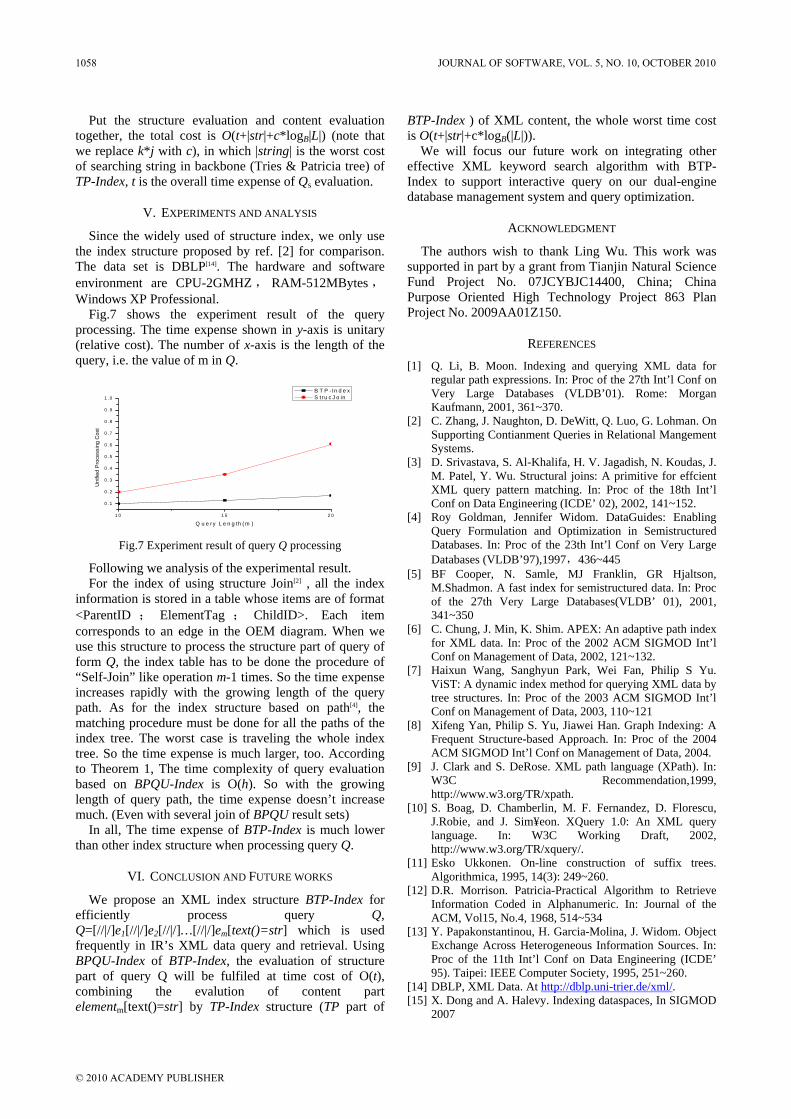
Fig.7 shows the experiment result of the query processing. The time expense shown in y-axis is unitary (relative cost). The number of x-axis is the length of the query, i.e. the value of m in Q.

1 0 1 5 2 0

0 .1

0 .2

0 .3

0 .4

0 .5

0 .6

0 .7

0 .8

0 .9

1 .0

Uni

fied

Pro

cess

ing

Cos

t

Q u e ry L e n g th ( m )

B T P - In d e x S tr u c J o in

Fig.7 Experiment result of query Q processing

Following we analysis of the experimental result. For the index of using structure Join[2] , all the index

information is stored in a table whose items are of format <ParentID ； ElementTag ； ChildID>. Each item corresponds to an edge in the OEM diagram. When we use this structure to process the structure part of query of form Q, the index table has to be done the procedure of “Self-Join” like operation m-1 times. So the time expense increases rapidly with the growing length of the query path. As for the index structure based on path[4], the matching procedure must be done for all the paths of the index tree. The worst case is traveling the whole index tree. So the time expense is much larger, too. According to Theorem 1, The time complexity of query evaluation based on BPQU-Index is O(h). So with the growing length of query path, the time expense doesn’t increase much. (Even with several join of BPQU result sets)

In all, The time expense of BTP-Index is much lower than other index structure when processing query Q.

VI. CONCLUSION AND FUTURE WORKS

We propose an XML index structure BTP-Index for efficiently process query Q, Q=[//|/]e1[//|/]e2[//|/]…[//|/]em[text()=str] which is used frequently in IR’s XML data query and retrieval. Using BPQU-Index of BTP-Index, the evaluation of structure part of query Q will be fulfiled at time cost of O(t), combining the evalution of content part elementm[text()=str] by TP-Index structure (TP part of

BTP-Index ) of XML content, the whole worst time cost is O(t+|str|+c*logB(|L|)).

We will focus our future work on integrating other effective XML keyword search algorithm with BTP-Index to support interactive query on our dual-engine database management system and query optimization.

ACKNOWLEDGMENT

The authors wish to thank Ling Wu. This work was supported in part by a grant from Tianjin Natural Science Fund Project No. 07JCYBJC14400, China; China Purpose Oriented High Technology Project 863 Plan Project No. 2009AA01Z150.

REFERENCES

[1] Q. Li, B. Moon. Indexing and querying XML data for regular path expressions. In: Proc of the 27th Int’l Conf on Very Large Databases (VLDB’01). Rome: Morgan Kaufmann, 2001, 361~370.

[2] C. Zhang, J. Naughton, D. DeWitt, Q. Luo, G. Lohman. On Supporting Contianment Queries in Relational Mangement Systems.

[3] D. Srivastava, S. Al-Khalifa, H. V. Jagadish, N. Koudas, J. M. Patel, Y. Wu. Structural joins: A primitive for effcient XML query pattern matching. In: Proc of the 18th Int’l Conf on Data Engineering (ICDE’ 02), 2002, 141~152.

[4] Roy Goldman, Jennifer Widom. DataGuides: Enabling Query Formulation and Optimization in Semistructured Databases. In: Proc of the 23th Int’l Conf on Very Large Databases (VLDB’97),1997，436~445

[5] BF Cooper, N. Samle, MJ Franklin, GR Hjaltson, M.Shadmon. A fast index for semistructured data. In: Proc of the 27th Very Large Databases(VLDB’ 01), 2001, 341~350

[6] C. Chung, J. Min, K. Shim. APEX: An adaptive path index for XML data. In: Proc of the 2002 ACM SIGMOD Int’l Conf on Management of Data, 2002, 121~132.

[7] Haixun Wang, Sanghyun Park, Wei Fan, Philip S Yu. ViST: A dynamic index method for querying XML data by tree structures. In: Proc of the 2003 ACM SIGMOD Int’l Conf on Management of Data, 2003, 110~121

[8] Xifeng Yan, Philip S. Yu, Jiawei Han. Graph Indexing: A Frequent Structure-based Approach. In: Proc of the 2004 ACM SIGMOD Int’l Conf on Management of Data, 2004.

[9] J. Clark and S. DeRose. XML path language (XPath). In: W3C Recommendation,1999, http://www.w3.org/TR/xpath.

[10] S. Boag, D. Chamberlin, M. F. Fernandez, D. Florescu, J.Robie, and J. Sim¥eon. XQuery 1.0: An XML query language. In: W3C Working Draft, 2002, http://www.w3.org/TR/xquery/.

[11] Esko Ukkonen. On-line construction of suffix trees. Algorithmica, 1995, 14(3): 249~260.

[12] D.R. Morrison. Patricia-Practical Algorithm to Retrieve Information Coded in Alphanumeric. In: Journal of the ACM, Vol15, No.4, 1968, 514~534

[13] Y. Papakonstantinou, H. Garcia-Molina, J. Widom. Object Exchange Across Heterogeneous Information Sources. In: Proc of the 11th Int’l Conf on Data Engineering (ICDE’ 95). Taipei: IEEE Computer Society, 1995, 251~260.

[14] DBLP, XML Data. At http://dblp.uni-trier.de/xml/. [15] X. Dong and A. Halevy. Indexing dataspaces, In SIGMOD

2007



[16] Daniela Florescu, Donald Kossmann, Ioana Manolescu: Integrating keyword search into XML query processing. Computer Networks (CN) 33(1-6):119-135 (2000)

[17] Lin Guo, Feng Shao, Chavdar Botev, Jayavel Shanmugasundaram: XRANK: Ranked Keyword Search over XML Documents. SIGMOD 2003:16-27

[18] Yu Xu, Yannis Papakonstantinou: Efficient Keyword Search for Smallest LCAs in XML Databases. SIGMOD 2005:537-538

[19] Andrey Balmin, Vagelis Hristidis, Nick Koudas, Yannis Papakonstantinou, Divesh Srivastava, Tianqiu Wang: A System for Keyword Proximity Search on XML Databases. VLDB 2003:1069-1072

[20] Vagelis Hristidis, Yannis Papakonstantinou, Andrey Balmin: Keyword Proximity Search on XML Graphs. ICDE 2003:367-378

[21] Mayssam Sayyadian, Hieu LeKhac, AnHai Doan, Luis Gravano: Efficient Keyword Search Across Heterogeneous Relational Databases. ICDE 2007:346-355

[22] V. Hristidis and Y. Papakonstantinou. DISCOVER: Keyword search in relational databases. In VLDB, 2002

[23] Kamal Taha, Ramez Elmasri: KSRQuerying: XML Keyword with Recursive Querying. XSym 2009:33-52

[24] Jiang Li, Junhu Wang, Mao Lin Huang: : effective and efficient keyword search in XML databases. IDEAS 2009:121-130

[25] Ziyang Liu, Yi Chen: Answering Keyword Queries on XML Using Materialized Views. ICDE 2008:1501-1503

Yanzhong Jin, 7/4/1972, Lanzhou, China. Master, physics, North West Normal Univ., Lanzhou, China, 1995; Post-graduate, computer science, Lanzhou Univ., China, 2000.

She works in Tianjin Sci.&Tech. Univ., Tianjin, China, Teacher. Her research interests includes XML data management,

database system, and software engineering. Publication: [1]ArithBi+ --An XML Index Structure on Reverse

Arithmetic Compressed XML Data, J.Computer Science, 2005(11)

She is a member of CCF(China Computer Federation).

Xiaoyuan Bao, 5/10/1971, Gansu, China. Master, physics, North West Normal Univ., Lanzhou, China, 1993; Post-graduate, computer science, Lanzhou Univ., Lanzhou, China, 1998; Doctor, computer science, Peking Univ. Beijing, China.

He work in Peking Univ., Beijing, China, Post-doctoral researcher. His research interests includes XML data

management, database system, and information retrival. Publications: [1]Bao Xiaoyuan, Tang Shiwei, Yang Dongqing. Interval+—

An Index Structure on Compressed XML Data Based on Interval Tree[J].Journal of Computer Research and Development, 2006(07).

[2]Bao Xiaoyuan, Tang Shiwei, Wu Ling, Yang Dongqing, Song Zaisheng, Wang Tengjiao. ArithRegion—An Index Structure on Compressed XML Data[J].Acta Scicentiarum Naturalium Universitatis Pekinesis, 2006(01).

[3]Bao Xiaoyuan, Tang Shiwei, Yang Dongqing, Song Zaisheng, Wang Tengjiao. BloomRouter: A Framework for Dissemination of Compressed XML Stream[J]. Acta Scicentiarum Naturalium Universitatis Wuhan, 2006(01).

He is a senior member of CCF.



Realtime and Embedded System Testing for Biomedical Applications

Jinhe Wang, Jing Zhao, Bing Yan

School of Computer Engineering, Qingdao Technological University, Qingdao, 266033, China [email protected]

Abstract—With realtime and embedded systems we propose a software testing approach to build a testing architecture for biomedical applications, it can check the reliability based on the failure data observed during software testing and can be applied to make the use of test task more flexible. The reliability of data of the system is computed through the test panel and simulation of the testing system by testing the reliabilities of the individual modules in the embedded system. One of the fundamental requirements for embedded system is the ability to obtain the testing data from command line of the program for process control in the testing system. Hence, the testing instructions can be formally described as a sequential decision commands in terms of their temperature, action time, incremental quantity and gradient. The testing approach has been applied in the system and achieved the testing requirements of the embedded system. Index Terms—Software testing, reliability, embedded system

I. INTRODUCTION

Embedded System have been developed in high speed, and used for many electronic devices in the field of routine diagnostics of biomedical applications. It performs a variety of functions for the users, and the complexity of embedded system is increased dramatically. Because of mass-production and fast time-to-market, the quality of product and overall cost has become important factors. The multi-level testing technique allows using partially defective logic and routing resources for normal operation, it spans over several engineering disciplines: mechanical engineering, electrical engineering and control engineering. There are many types and design methods for software testing in the Biomedical Embedded system, especially for temperature control testing [1-12]. The application of this method is focused on polymerase chain reaction embedded system, which has cycling reactions such as Denaturation, Annealing and extension [13-15]. Several different models have been designed and applied for testing in the field of basic research. The following sections will provide a description for the software testing on the realtime& embedded system. In Section II, we describe the architecture of the system testing. Finally, a brief conclusion is given in Section III.

II. THE ARCHITECTURE OF THE SYSTEM TESTING

The embedded system is for a gene amplification system consisting of data sampling, heat execution, man-

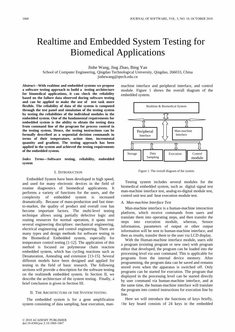
machine interface and peripheral interface, and control module. Figure 1 shows the overall diagram of the embedded system.

Testing system includes several modules for the biomedical embedded system, such as digital signal test man-machine interface test, analog-to-digital module test, control unit test and heat execution module test.

A. Man-machine Interface Test Man-machine interface is a human-machine interaction

platform, which receive commands from users and translate them into operating steps, and then transfer the steps into execution module, whereas, Sensor information, parameters of output or other output informaiton will be sent to human-machine interface, and then as results, transfer them to the user via LCD display.

With the Human-machine interface module, users edit a program (existing program or new one) with program editor that developed, the program can be loaded into the processing level via user command. This is applicable for programs from the internal device memory. After programming, the program data can be saved and remains stored even when the apparatus is switched off. Only programs can be started for execution. The program that displayed in the processing level can be started directly by user command via human-machine interface, and at the same time, the human-machine interface will translate the program into control instructions for execution line by line.

Here we will introduce the functions of keys briefly, the key board consists of 24 keys in the embedded

Figure 1. The overall diagram of the system.

Peripheral Interface

Realtime & Biomedical System

Data Sampling

Execution Control module

Man-machine Interface

Storage



system, they are programming keys, cursor/confirm keys, control keys, file key, setting key, reverse key and 10 digital keys.

The programming key consists of Ins Key, Del Key and Exit Key; cursor/confirm key consists of Left key, Right key, Up key, Down key and Confirm key; Control key includes Start key, Stop key and Pause key.

Let us take the programming key as an example: During the creation of a program, program lines can be inserted by pressing Ins Key, or they would be deleted by pressing Del Key.

In order to test the program executed in the Man-machine interface module, a test system is designed, the panel of the system is show as Figure 2, There are 40 lights on the panel, the first light-line includes 20 lights, which named LED1, LED2, LED3, …, LED20 respectively, the second light-line includes 10 lights, the names of these lights are LED21, LED22, LED23, …, LED30, and the third includes LED31, LED32, LED33, …, LED40.

There three software testing tasks for Man-machine

interface module. 1 Key-board Test Keys on the key-board are pointed to their very LEDs

on the test panel , the relationship between keys and LEDs is shown in Table I.

The steps for testing task are as following:

Step 1. connect the 40-pin cable to the hardware of the embedded system and the test panel

Step 2. connect the 4-pin cable to the hardware of the embedded system and the test panel

Step 3. start testing the program of man-machine interface

Step 4. For each testing key, it corresponds to one of the LEDs shown in Table I, press the key, if the

LED fails to light, the key, functions with the key, or the program codes edited for the key should be checked properly.

Step 5. End.

Special test for keys: In order to avoid the twice times or more between a

given interval when a key is pressed, the testing strategy let the corresponding LED to be triggered many times when the phenomenon occurs.

2 Command-line Test A program edited for the embedded system contains

two basic commands for controlling the temperature of the thermal block and of the heated lid as well as seven different command lines for programming. A program can contain up to 200 program lines. The command-lines (CML) may be repeated as desired. Digits or letters may be pressed via key board. Selections should be made for

Figure 2. The test panel of the system

TABLE I. THE RELATIONSHIP BETWEEN KEYS AND LEDS

Type Relationship

Description LED

Programming keys

Ins Key LED1

Del Key LED2

Exit Key LED3

Cursor/confirm key

Left key LED4

Right key LED5

Up key LED6

Down key LED7

Confirm key LED8

Control key

Start key LED9

Stop key LED10

Pause key LED11

Digital Key

0-key LED12

1-key LED13

2-key LED14

3-key LED15

4-key LED16

5-key LED17

6-key LED18

7-key LED19

8-key LED20

9-key LED21

Other key

File key LED22

Setting key LED23

Reverse key LED24



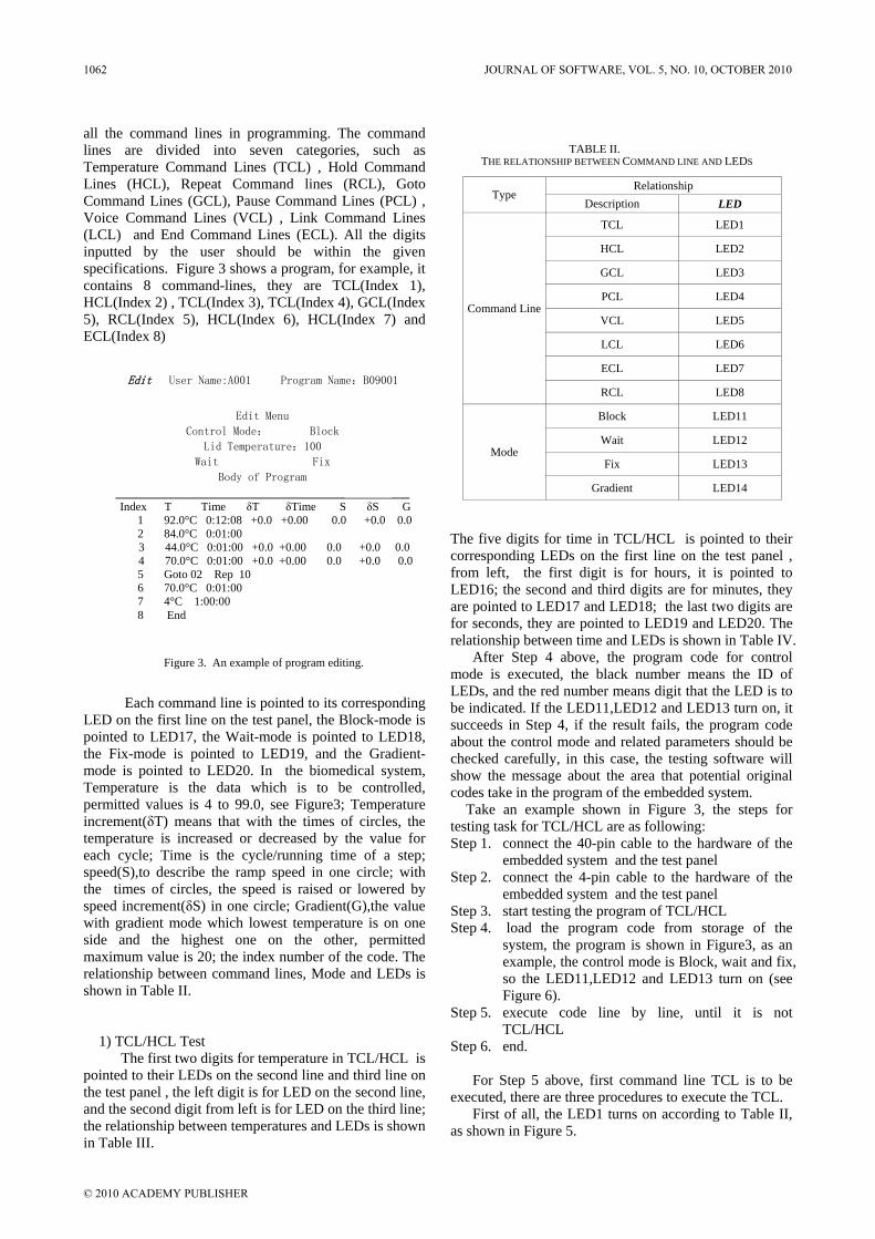
all the command lines in programming. The command lines are divided into seven categories, such as Temperature Command Lines (TCL) , Hold Command Lines (HCL), Repeat Command lines (RCL), Goto Command Lines (GCL), Pause Command Lines (PCL) , Voice Command Lines (VCL) , Link Command Lines (LCL) and End Command Lines (ECL). All the digits inputted by the user should be within the given specifications. Figure 3 shows a program, for example, it contains 8 command-lines, they are TCL(Index 1), HCL(Index 2) , TCL(Index 3), TCL(Index 4), GCL(Index 5), RCL(Index 5), HCL(Index 6), HCL(Index 7) and ECL(Index 8)

Each command line is pointed to its corresponding

LED on the first line on the test panel, the Block-mode is pointed to LED17, the Wait-mode is pointed to LED18, the Fix-mode is pointed to LED19, and the Gradient-mode is pointed to LED20. In the biomedical system, Temperature is the data which is to be controlled, permitted values is 4 to 99.0, see Figure3; Temperature increment(δT) means that with the times of circles, the temperature is increased or decreased by the value for each cycle; Time is the cycle/running time of a step; speed(S),to describe the ramp speed in one circle; with the times of circles, the speed is raised or lowered by speed increment(δS) in one circle; Gradient(G),the value with gradient mode which lowest temperature is on one side and the highest one on the other, permitted maximum value is 20; the index number of the code. The relationship between command lines, Mode and LEDs is shown in Table II.

1) TCL/HCL Test The first two digits for temperature in TCL/HCL is

pointed to their LEDs on the second line and third line on the test panel , the left digit is for LED on the second line, and the second digit from left is for LED on the third line; the relationship between temperatures and LEDs is shown in Table III.

The five digits for time in TCL/HCL is pointed to their corresponding LEDs on the first line on the test panel , from left, the first digit is for hours, it is pointed to LED16; the second and third digits are for minutes, they are pointed to LED17 and LED18; the last two digits are for seconds, they are pointed to LED19 and LED20. The relationship between time and LEDs is shown in Table IV.

After Step 4 above, the program code for control mode is executed, the black number means the ID of LEDs, and the red number means digit that the LED is to be indicated. If the LED11,LED12 and LED13 turn on, it succeeds in Step 4, if the result fails, the program code about the control mode and related parameters should be checked carefully, in this case, the testing software will show the message about the area that potential original codes take in the program of the embedded system.

Take an example shown in Figure 3, the steps for testing task for TCL/HCL are as following: Step 1. connect the 40-pin cable to the hardware of the

embedded system and the test panel Step 2. connect the 4-pin cable to the hardware of the

embedded system and the test panel Step 3. start testing the program of TCL/HCL Step 4. load the program code from storage of the

system, the program is shown in Figure3, as an example, the control mode is Block, wait and fix, so the LED11,LED12 and LED13 turn on (see Figure 6).

Step 5. execute code line by line, until it is not TCL/HCL

Step 6. end.

For Step 5 above, first command line TCL is to be executed, there are three procedures to execute the TCL.

First of all, the LED1 turns on according to Table II, as shown in Figure 5.

TABLE II. THE RELATIONSHIP BETWEEN COMMAND LINE AND LEDS

Type Relationship

Description LED

Command Line

TCL LED1

HCL LED2

GCL LED3

PCL LED4

VCL LED5

LCL LED6

ECL LED7

RCL LED8

Mode

Block LED11

Wait LED12

Fix LED13

Gradient LED14

Figure 3. An example of program editing.

Edit User Name:A001 Program Name：B09001

Edit Menu

Control Mode： Block

Lid Temperature：100

Wait Fix

Body of Program

_______________________________________ ___ Index T Time δT δTime S δS G

1 92.0°C 0:12:08 +0.0 +0.00 0.0 +0.0 0.0 2 84.0°C 0:01:00

3 44.0°C 0:01:00 +0.0 +0.00 0.0 +0.0 0.0 4 70.0°C 0:01:00 +0.0 +0.00 0.0 +0.0 0.0

5 Goto 02 Rep 10 6 70.0°C 0:01:00 7 4°C 1:00:00 8 End



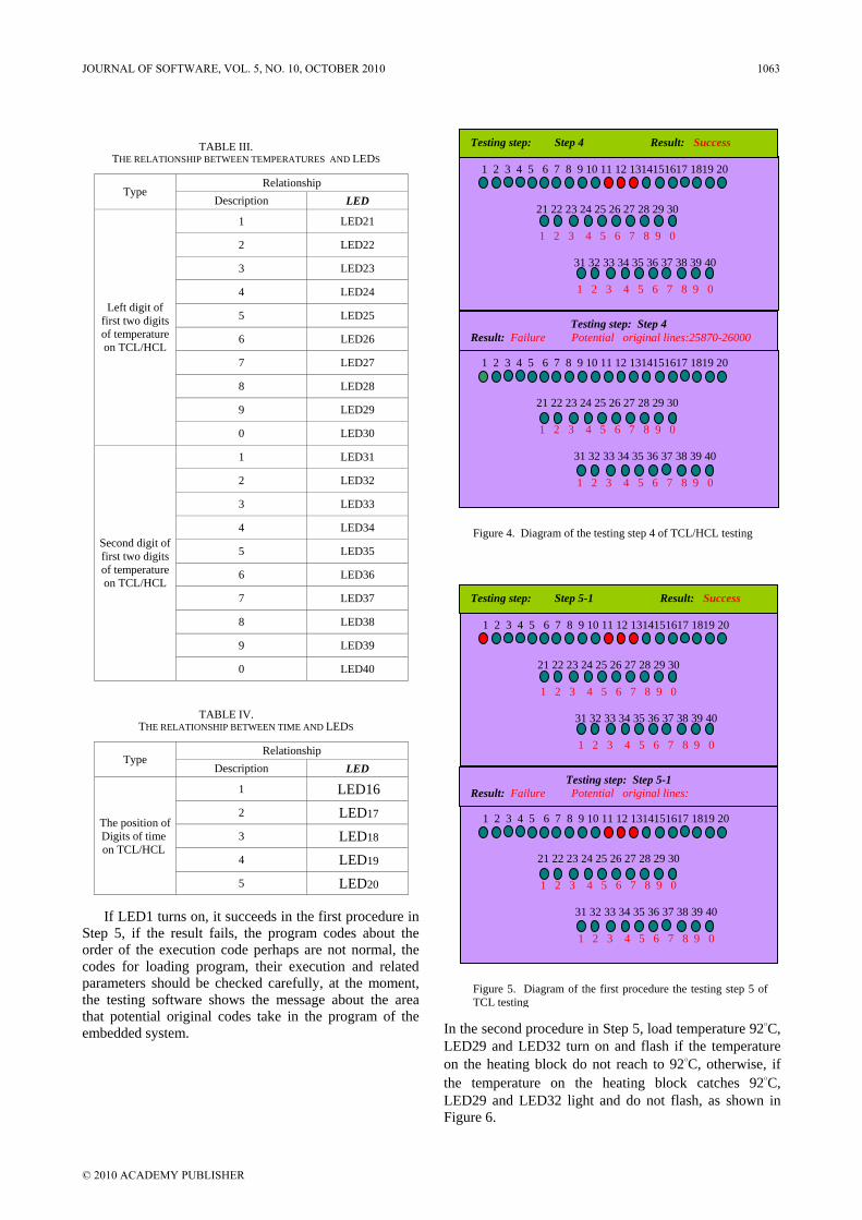
If LED1 turns on, it succeeds in the first procedure in

Step 5, if the result fails, the program codes about the order of the execution code perhaps are not normal, the codes for loading program, their execution and related parameters should be checked carefully, at the moment, the testing software shows the message about the area that potential original codes take in the program of the embedded system.

In the second procedure in Step 5, load temperature 92oC, LED29 and LED32 turn on and flash if the temperature on the heating block do not reach to 92oC, otherwise, if the temperature on the heating block catches 92oC, LED29 and LED32 light and do not flash, as shown in Figure 6.

Figure 4. Diagram of the testing step 4 of TCL/HCL testing

1 2 3 4 5 6 7 8 9 10 11 12 1314151617 1819 20

21 22 23 24 25 26 27 28 29 30 1 2 3 4 5 6 7 8 9 0 31 32 33 34 35 36 37 38 39 40 1 2 3 4 5 6 7 8 9 0

Testing step: Step 4 Result: Success

Testing step: Step 4 Result: Failure Potential original lines:25870-26000

1 2 3 4 5 6 7 8 9 10 11 12 1314151617 1819 20

21 22 23 24 25 26 27 28 29 30 1 2 3 4 5 6 7 8 9 0 31 32 33 34 35 36 37 38 39 40 1 2 3 4 5 6 7 8 9 0

TABLE IV. THE RELATIONSHIP BETWEEN TIME AND LEDS

Type Relationship

Description LED

The position of Digits of time on TCL/HCL

1 LED16

2 LED17

3 LED18

4 LED19

5 LED20

TABLE III. THE RELATIONSHIP BETWEEN TEMPERATURES AND LEDS

Type Relationship

Description LED

Left digit of first two digits of temperature on TCL/HCL

1 LED21

2 LED22

3 LED23

4 LED24

5 LED25

6 LED26

7 LED27

8 LED28

9 LED29

0 LED30

Second digit of first two digits of temperature on TCL/HCL

1 LED31

2 LED32

3 LED33

4 LED34

5 LED35

6 LED36

7 LED37

8 LED38

9 LED39

0 LED40

Figure 5. Diagram of the first procedure the testing step 5 of TCL testing

1 2 3 4 5 6 7 8 9 10 11 12 1314151617 1819 20

21 22 23 24 25 26 27 28 29 30 1 2 3 4 5 6 7 8 9 0 31 32 33 34 35 36 37 38 39 40 1 2 3 4 5 6 7 8 9 0

Testing step: Step 5-1 Result: Success

Testing step: Step 5-1 Result: Failure Potential original lines:

1 2 3 4 5 6 7 8 9 10 11 12 1314151617 1819 20

21 22 23 24 25 26 27 28 29 30 1 2 3 4 5 6 7 8 9 0 31 32 33 34 35 36 37 38 39 40 1 2 3 4 5 6 7 8 9 0



It succeeds in the second procedure in Step 5 (above in Figure 6), if the result fails, the LED29 turns off or LED32 off, the program codes about the loading of the temperature are not normal, as shown in Figure 6, the codes for loading program, the codes for execution and

related parameters should be checked carefully, at the moment, the testing software will show the message about the area that potential original codes take in the program of the embedded system.

In the third procedure in Step 5, load time, 0:12:08, LED17, LED18 and LED20 turn on and flash, the data of the time decreases with the running of the procedure, LED17, LED18 and LED20 indicate the position of the digit of the time (hour, minute, or second). If not all of the LED17, LED18 and LED20 turn on at the first stage of the third procedure in Step 5 ,as shown in Figure 7, the result fails, the program codes about the load of the data code are not correct, the codes for loading program, their execution and related parameters should be checked carefully.

The second command line is HCL in Step 5, it is similar to the first command line, it is to be executed by three procedures, too.

Figure 8 shows the third procedure to execute the HCL in Step 5, No error occurs in this procedure.

2) GCL/RCL Test The steps for testing task for GCL/RCL are as

following: Step 1. start testing the program of GCL/RCL Step 2. load the program code from storage of the

system Step 3. execute GCL/RCL code Step 4. end.

For Step 3, it is similar to the TCL/HCL testing, it is to be executed by two procedures.

Figure 9 shows the second procedure to execute the GCL in Step 3, No error occurs in this procedure.

Figure 8. Diagram of the third procedure to execute HCL in the testing step 5

1 2 3 4 5 6 7 8 9 10 11 12 1314151617 1819 20

21 22 23 24 25 26 27 28 29 30 1 2 3 4 5 6 7 8 9 0 31 32 33 34 35 36 37 38 39 40 1 2 3 4 5 6 7 8 9 0


Testing step: Step 5-3 Result: Success Potential original lines:No

1 2 3 4 5 6 7 8 9 10 11 12 1314151617 1819 20

21 22 23 24 25 26 27 28 29 30 1 2 3 4 5 6 7 8 9 0 31 32 33 34 35 36 37 38 39 40 1 2 3 4 5 6 7 8 9 0

Figure 7. Diagram of the third procedure in the testing step 5 of TCL testing

1 2 3 4 5 6 7 8 9 10 11 12 1314151617 1819 20

21 22 23 24 25 26 27 28 29 30 1 2 3 4 5 6 7 8 9 0 31 32 33 34 35 36 37 38 39 40 1 2 3 4 5 6 7 8 9 0

1 2 3 4 5 6 7 8 9 10 11 12 1314151617 1819 20

21 22 23 24 25 26 27 28 29 30 1 2 3 4 5 6 7 8 9 0 31 32 33 34 35 36 37 38 39 40 1 2 3 4 5 6 7 8 9 0



Figure 6. Diagram of the second procedure in the testing step 5 of TCL testing

1 2 3 4 5 6 7 8 9 10 11 12 1314151617 1819 20

21 22 23 24 25 26 27 28 29 30 1 2 3 4 5 6 7 8 9 0 31 32 33 34 35 36 37 38 39 40 1 2 3 4 5 6 7 8 9 0

1 2 3 4 5 6 7 8 9 10 11 12 1314151617 1819 20

21 22 23 24 25 26 27 28 29 30 1 2 3 4 5 6 7 8 9 0 31 32 33 34 35 36 37 38 39 40 1 2 3 4 5 6 7 8 9 0





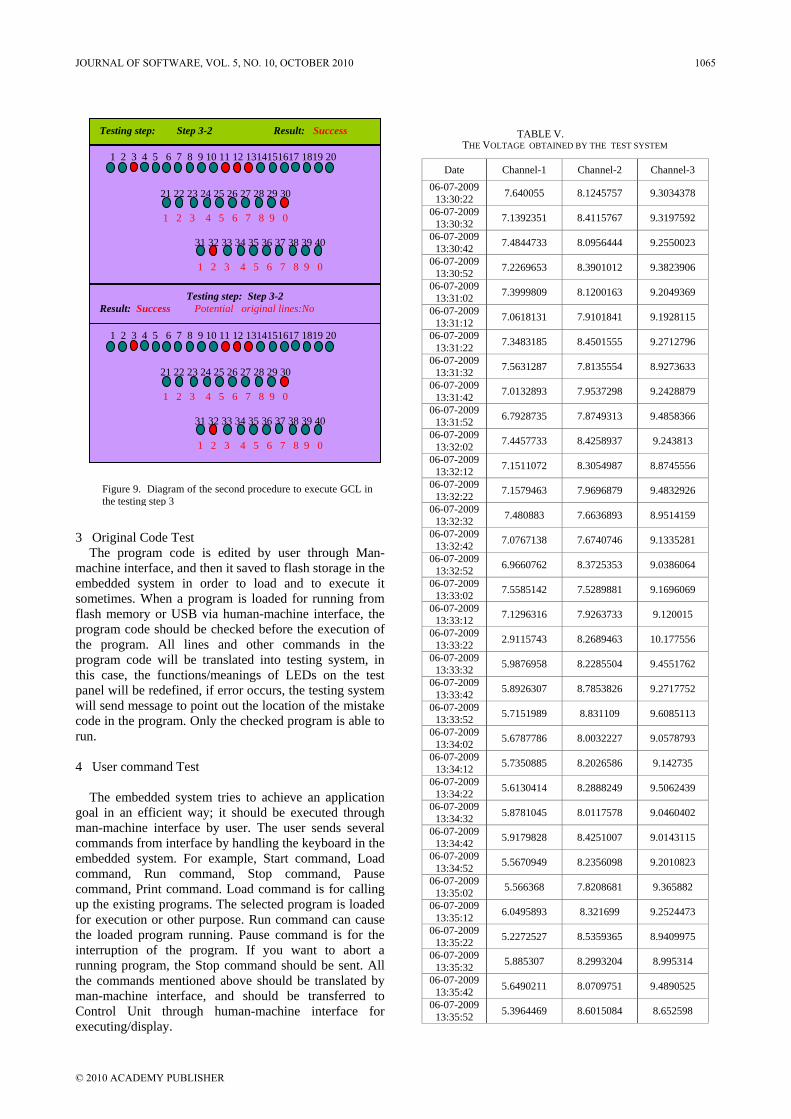
3 Original Code Test

The program code is edited by user through Man-machine interface, and then it saved to flash storage in the embedded system in order to load and to execute it sometimes. When a program is loaded for running from flash memory or USB via human-machine interface, the program code should be checked before the execution of the program. All lines and other commands in the program code will be translated into testing system, in this case, the functions/meanings of LEDs on the test panel will be redefined, if error occurs, the testing system will send message to point out the location of the mistake code in the program. Only the checked program is able to run. 4 User command Test

The embedded system tries to achieve an application

goal in an efficient way; it should be executed through man-machine interface by user. The user sends several commands from interface by handling the keyboard in the embedded system. For example, Start command, Load command, Run command, Stop command, Pause command, Print command. Load command is for calling up the existing programs. The selected program is loaded for execution or other purpose. Run command can cause the loaded program running. Pause command is for the interruption of the program. If you want to abort a running program, the Stop command should be sent. All the commands mentioned above should be translated by man-machine interface, and should be transferred to Control Unit through human-machine interface for executing/display.

Figure 9. Diagram of the second procedure to execute GCL in the testing step 3

1 2 3 4 5 6 7 8 9 10 11 12 1314151617 1819 20

21 22 23 24 25 26 27 28 29 30 1 2 3 4 5 6 7 8 9 0 31 32 33 34 35 36 37 38 39 40 1 2 3 4 5 6 7 8 9 0


Testing step: Step 3-2 Result: Success Potential original lines:No

1 2 3 4 5 6 7 8 9 10 11 12 1314151617 1819 20

21 22 23 24 25 26 27 28 29 30 1 2 3 4 5 6 7 8 9 0 31 32 33 34 35 36 37 38 39 40 1 2 3 4 5 6 7 8 9 0

TABLE V. THE VOLTAGE OBTAINED BY THE TEST SYSTEM

Date Channel-1 Channel-2 Channel-3 06-07-2009

13:30:22 7.640055 8.1245757 9.3034378

06-07-2009 13:30:32 7.1392351 8.4115767 9.3197592

06-07-2009 13:30:42 7.4844733 8.0956444 9.2550023

06-07-2009 13:30:52 7.2269653 8.3901012 9.3823906

06-07-2009 13:31:02 7.3999809 8.1200163 9.2049369

06-07-2009 13:31:12 7.0618131 7.9101841 9.1928115

06-07-2009 13:31:22 7.3483185 8.4501555 9.2712796

06-07-2009 13:31:32 7.5631287 7.8135554 8.9273633

06-07-2009 13:31:42 7.0132893 7.9537298 9.2428879

06-07-2009 13:31:52 6.7928735 7.8749313 9.4858366

06-07-2009 13:32:02 7.4457733 8.4258937 9.243813

06-07-2009 13:32:12 7.1511072 8.3054987 8.8745556

06-07-2009 13:32:22 7.1579463 7.9696879 9.4832926

06-07-2009 13:32:32 7.480883 7.6636893 8.9514159

06-07-2009 13:32:42 7.0767138 7.6740746 9.1335281

06-07-2009 13:32:52 6.9660762 8.3725353 9.0386064

06-07-2009 13:33:02 7.5585142 7.5289881 9.1696069

06-07-2009 13:33:12 7.1296316 7.9263733 9.120015

06-07-2009 13:33:22 2.9115743 8.2689463 10.177556

06-07-2009 13:33:32 5.9876958 8.2285504 9.4551762

06-07-2009 13:33:42 5.8926307 8.7853826 9.2717752

06-07-2009 13:33:52 5.7151989 8.831109 9.6085113

06-07-2009 13:34:02 5.6787786 8.0032227 9.0578793

06-07-2009 13:34:12 5.7350885 8.2026586 9.142735

06-07-2009 13:34:22 5.6130414 8.2888249 9.5062439

06-07-2009 13:34:32 5.8781045 8.0117578 9.0460402

06-07-2009 13:34:42 5.9179828 8.4251007 9.0143115

06-07-2009 13:34:52 5.5670949 8.2356098 9.2010823

06-07-2009 13:35:02 5.566368 7.8208681 9.365882

06-07-2009 13:35:12 6.0495893 8.321699 9.2524473

06-07-2009 13:35:22 5.2272527 8.5359365 8.9409975

06-07-2009 13:35:32 5.885307 8.2993204 8.995314

06-07-2009 13:35:42 5.6490211 8.0709751 9.4890525

06-07-2009 13:35:52 5.3964469 8.6015084 8.652598



The task of testing procedure is to find out the mistakes or other potential errors before executing such commands, for each command in the system, there are special definitions with test panel, and it performs such interactions with the user efficiently.

B. Data sampling module Test Data sampling module is very important in this system,

Signals from this module are amplified, filtered, and the analogy signals should be converted into digital signals before imported into the Control Unit.

In this paper, the test task of the data sampling module includes the multi-channels data testing, and filtration test. The test panel should be redefined when applied in this module, the first 20 LEDs (from LED1 to LED 20) is for signals imported through 20-pin cable from the module, and other LEDs indicate the states of the module.In this data sampling system, interleaving multiple analog-to-digital converters is performed with the intent to increase a converters effective sample rate, however, time-interleaving data converters is not an easy task, because the offset mismatches and timing errors can cause undesired spurs in the spectrum of the system. Therefore, you wouldn't gain a good performance for the temperature control without excellent data sampling system. The test system can automatically set the sampling parameter such as sampling channel and sampling frequency, and the results show that the test system has good performance in the testing procedure.

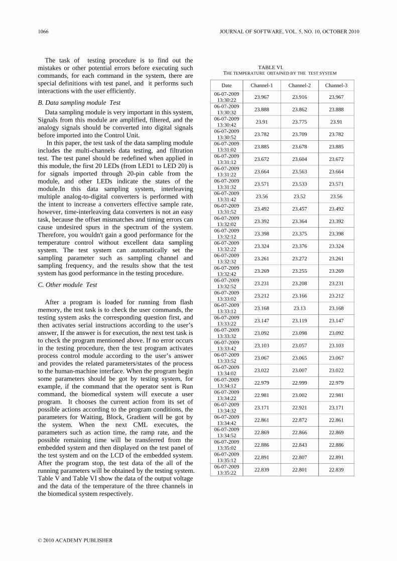
C. Other module Test

After a program is loaded for running from flash memory, the test task is to check the user commands, the testing system asks the corresponding question first, and then activates serial instructions according to the user’s answer, If the answer is for execution, the next test task is to check the program mentioned above. If no error occurs in the testing procedure, then the test program activates process control module according to the user’s answer and provides the related parameters/states of the process to the human-machine interface. When the program begin some parameters should be got by testing system, for example, if the command that the operator sent is Run command, the biomedical system will execute a user program. It chooses the current action from its set of possible actions according to the program conditions, the parameters for Waiting, Block, Gradient will be got by the system. When the next CML executes, the parameters such as action time, the ramp rate, and the possible remaining time will be transferred from the embedded system and then displayed on the test panel of the test system and on the LCD of the embedded system. After the program stop, the test data of the all of the running parameters will be obtained by the testing system. Table V and Table VI show the data of the output voltage and the data of the temperature of the three channels in the biomedical system respectively.

TABLE VI. THE TEMPERATURE OBTAINED BY THE TEST SYSTEM

Date Channel-1 Channel-2 Channel-3 06-07-2009

13:30:22 23.967 23.916 23.967

06-07-2009 13:30:32 23.888 23.862 23.888

06-07-2009 13:30:42 23.91 23.775 23.91

06-07-2009 13:30:52 23.782 23.709 23.782

06-07-2009 13:31:02 23.885 23.678 23.885

06-07-2009 13:31:12 23.672 23.604 23.672

06-07-2009 13:31:22 23.664 23.563 23.664

06-07-2009 13:31:32 23.571 23.533 23.571

06-07-2009 13:31:42 23.56 23.52 23.56

06-07-2009 13:31:52 23.492 23.457 23.492

06-07-2009 13:32:02 23.392 23.364 23.392

06-07-2009 13:32:12 23.398 23.375 23.398

06-07-2009 13:32:22 23.324 23.376 23.324

06-07-2009 13:32:32 23.261 23.272 23.261

06-07-2009 13:32:42 23.269 23.255 23.269

06-07-2009 13:32:52 23.231 23.208 23.231

06-07-2009 13:33:02 23.212 23.166 23.212

06-07-2009 13:33:12 23.168 23.13 23.168

06-07-2009 13:33:22 23.147 23.119 23.147

06-07-2009 13:33:32 23.092 23.098 23.092

06-07-2009 13:33:42 23.103 23.057 23.103

06-07-2009 13:33:52 23.067 23.065 23.067

06-07-2009 13:34:02 23.022 23.007 23.022

06-07-2009 13:34:12 22.979 22.999 22.979

06-07-2009 13:34:22 22.981 23.002 22.981

06-07-2009 13:34:32 23.171 22.921 23.171

06-07-2009 13:34:42 22.861 22.872 22.861

06-07-2009 13:34:52 22.869 22.866 22.869

06-07-2009 13:35:02 22.886 22.843 22.886

06-07-2009 13:35:12 22.891 22.807 22.891

06-07-2009 13:35:22 22.839 22.801 22.839



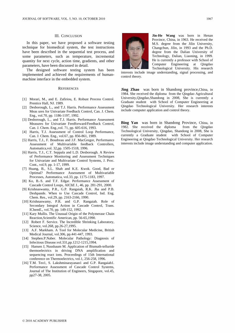
III. CONCLUSION

In this paper, we have proposed a software testing technique for biomedical system, the test instructions have been described in the sequential test process, and some parameters, such as temperature, incremental quantity for next cycle, action time, gradients, and other parameters, have been discussed in detail.

The designed software testing system has been implemented and achieved the requirements of human-machine interface in the embedded system.

REFERENCES

[1] Morari, M., and E. Zafiriou, E. Robust Process Control.

Prentice Hall, NJ. 1989. [2] Desborough, L., and T.J. Harris. Performance Assessment

Meas ures for Univariate Feedback Control, Can. J. Chem. Eng., vol.70, pp. 1186-1197, 1992.

[3] Desborough, L., and T.J. Harris. Performance Assessment Measures for Univariate Feedforward/Feedback Control, Can. J. Chem. Eng.,vol. 71, pp. 605-616, 1993.

[4] Harris, T.J. Assessment of Control Loop Performance, Can. J. Chem. Eng., vol.67, pp. 856-861, 1989.

[5] Harris, T.J., F. Boudreau and J.F. MacGregor, Performance Assessment of Multivariable feedback Controllers, Automatica,vol. 32,pp. 1505-1518, 1996.

[6] Harris, T.J., C.T. Seppala and L.D. Desborough. A Review of Performance Monitoring and Assessment Techniques for Univariate and Multivariate Control Systems, J. Proc. Cont., vol.9, pp. 1-17, 1999.

[7] Huang, B., S.L. Shah and K.E. Kwok. Good, Bad or Optimal? Performance Assessment of Multivariable Processes, Automatica, vol.33, pp. 1175-1183, 1997.

[8] Ko, B.-S. and T.F. Edgar. Performance Assessment of Cascade Control Loops, AIChE J., 46, pp. 281-291, 2000.

[9] Krishnaswamy, P.R., G.P. Rangaiah, R.K. Jha and P.B. Deshpande. When to Use Cascade Control, Ind. Eng. Chem. Res., vol.29, pp. 2163-2166, 1990.

[10] Krishnaswamy, P.R. and G.P. Rangaiah. Role of Secondary Integral Action in Cascade Control, Trans. IChemE., vol.70, pp. 149-152, 1992.

[11] Kary Mullis. The Unusual Origin of the Polymerase Chain Reaction,Scientific American, pp. 56-65,1990.

[12] Robert F. Service. The Incredible Shrinking Laboratory, Science, vol.268, pp.26-27,1995.

[13] A.F. Markham. A Tool for Molecular Medicine, British Medical Journal, vol.306, pp.441-447, 1993.

[14] Stephen.P.Naber. Molecular Pathology: Diagnosis of Infectious Disease.vol.331,pp.1212-1215,1994.

[15] Hansen J, Nussbaum M. Application of Bismuth-telluride thermoelectrics in driving DNA amplification and sequencing react ions. Proceedings of 15th International conference on Thermoelectrics, vol.1, 256-258, 1996.

[16] T.M. Teo1, S. Lakshminarayanan1 and G.P. Rangaiah1. Performance Assessment of Cascade Control Systems, Journal of The Institution of Engineers, Singapore, vol.45, pp27-38, 2005.

Jin-He Wang was born in Henan Province, China, in 1963. He received the M.S. degree from the Jilin University, Changchun, Jilin, in 1993 and the Ph.D. degree from the Dalian University of Technology, Dalian, Liaoning, in 1999. He is currently a professor with School of Computer Engineering at Qingdao Technological University. His research

interests include image understanding, signal processing, and control theory. Jing Zhao was born in Shandong province,China, in 1984. She received the diploma from the Qingdao Agricultural University,Qingdao,Shandong in 2008, She is currently a Graduate student with School of Computer Engineering at Qingdao Technological University. Her research interests include computer application and control theory. Bing Yan was born in Shandong Province, China, in 1982. She received the diploma from the Qingdao Technological University, Qingdao, Shandong in 2008, She is currently a Graduate student with School of Computer Engineering at Qingdao Technological University. Her research interests include image understanding and computer application.



Color Map and Polynomial Coefficient Map Mapping

Huijian Han School of Computer Science & Technology, Shandong University, Jinan ,China

School of Computer Science & Technology, Shandong Economic University, Jinan ,China

Shandong Prov. Key Lab of Digital Media Technology, Jinan ,China Email: [email protected]

Caiming Zhang

School of Computer Science & Technology, ShanDong Economic University, Jinan ,China School of Computer Science & Technology, ShanDong University, Jinan ,China

Shandong Prov. Key Lab of Digital Media Technology, Jinan ,China Email: [email protected]

Abstract—In computer graphics, texture mapping is an important means to enhance the realism of model. Traditional texture image always was captured under special light condition. If the lighting in virtual environment is different from the texture image, the result of rendering will be incorrect and unrealistic. This paper proposes an image-based method to fit the reflection mode by a quadratic multinomial. The coefficients of quadratic multinomial will be gained from BTFs and are stored for every texel as polynomial coefficient maps. A picture is taken under well-proportioned environment light as a color map, which the chromaticity is saved. The method can interpolate light effective under varying virtual lighting conditions by color map and coefficient maps and represent the variation of luminance and color for each texel independently. Color map and polynomial coefficient map make texture mapping become more realistic, simple and dynamic. Index Terms—color map, polynomial coefficient map, iamge-based , texture mapping

I. INTRODUCTION

In the reality scene, there are three basic structures in the geometry, namely macrostructure, mesostructure and microstructure. The macrostructure with the certain geometry shape can be seen by the eyes, such as building, furniture shape etc. Mesostructure with quite small geometry shape still can be seen, for instance orange’s skin. Microstructure is the micro unit of surface can’t be seen. The Microstructure affects optical quality such as light scattering. The mesostructure causes visual effect [1] like roughness, self-shadows, occlusions, inter-reflection and subsurface scatting etc., which is an important factor that we get the realistic object surface with rich detail [2]. Mesostructures are typically rendered using techniques such as bump mapping [3], horizon mapping [4] or displacement mapping [5]. Mesostructure and microstructure decide the optical quality and the

detail visual quality of object surface. Using traditional texture, for example a realistic image,

may realistically increase the model’s geometry detail by mapping texture to the surface of object. However, because the texture is generally get by taking photographs under some special viewpoint position and specific lighting condition. When this texture is mapped to the 3-D object surface, the lighting condition in the virtual scene is not considered. If the lighting in the virtual environment is consistent with the lighting which the texture was captured under, the reality is the most strong. Contrarily, the result of rendering will appear incorrect and unrealistic. Bump mapping provides basic shading, which perturbs mesh normals to match those of the fine geometric detail, but not shadowing, occlusion, and silhouettes. Introducing variations in the surface normals causes the lighting method to render the surface as though it had local surface variations instead of just a smooth surface. Bump maps can be either hand modeled or, more typically, calculated procedurally. But it is still difficult to create a bump map base on real pictures.

This paper proposes an image-based method for representing various lighting effect, which is suitable for the diffuse and specular reflection object. The pictures are captured under fixed viewpoint and under kinds of illuminations condition. We choose a polynomial model to describe the variation of each texel’s luminance. The polynomial coefficients can be stored as polynomial coefficient maps. A picture is taken under well-proportioned environment light as a color map. The color map and polynomial coefficient maps can be mapped to the object simultaneously. This method can reconstruct the texture’s luminance and color under varying virtual lighting conditions.

II. TEXTURE LUMINANCE FITTING

A. Related work Many studies have contributed much to rendering real-

world objects in virtual space in high quality. An important problem is acquisition of reflection properties

Manuscript received Aug. 4, 2009; revised Aug. 20, 2009; acceptedAug. 30, 2009

Corresponding author: Huijian Han Email: [email protected]; [email protected] Adress : No.7366 ERHUAN Road, Jinan city, China, 250014



and geometric detail of surface. Geometry and reflection properties as textures mapped to the surface of 3D model can realistically reproduce an appearance of real world object.

Reflection model-based methods BRDFs(Bidirectional Reflectance Distribution

Function) were introduced by Nicodemus [6] which characterizes the color of a surface as a function of incident light and exitant view directions. There have been a large number of techniques developed to accurately and compactly represent the 4D BRDF. These include linear basis functions such as spherical harmonics [7], [8], [9], physically based analytic models [10], [11],and empirical models [12], [13]. Parametric-based methods emphasize the use of physically-based or empirical parametric reflectance models, which are effective abstraction for describing how the light is reflected from a surface. Often to fit reflection models based on a sparser set of samples. A number of researchers have described methods for fitting reflection models to measured sample data [14] [15] [13] [16] [17] [18] [19]. Of these methods, the ones by Ward Larson [18] and Lafortune et al. [13] do not consider spatial variations. Sato et al.[17] fit a Torrance-Sparrow model [20] to the data, and consider high-frequency variations for the diffuse part but only per-triangle variations for the specular part. This is also the case for the work by Yu et al. [19][21], which also takes indirect illumination into account. Boivin and Gagalowicz[22] reconstruct arbitrary reflection properties for whole patches in a scene using just one image. McAllister [16] fits a spatially varying Lafortune model to very densely sampled planar materials. The achieved results are impressive but the technique requires flat surfaces and an automated setup to get a dense sampling of the reflection properties. In [23] and [24] inverse rendering algorithms are proposed that reconstruct the reflection properties and the incident light field at the same time. Ramamoorthi and Hanrahan [23] as well as Westin et al. [25] project BRDF data into a spherical harmonics basis instead of fitting an explicit reflection model.

The traditional approach to measure reflectance properties is to use specialized devices, that position both a light source and a sensor relative to the material. These devices can only obtain one sample for each pair of light and sensor position and are therefore relatively slow. Image-sampling approaches have been proposed. These methods are able to acquire a large number of samples at once. For example, Ward Larson [18] uses a hemispherical mirror to sample the exitant hemisphere of light with a single image. Instead of using curved mirrors, it is also possible to use curved geometry to obtain a large number of samples with a single image. This approach is taken by Lu et al. [26], who assume a cylindrical surface, and Marschner et al. [27] who obtain the geometry using a range scanner.

Image-Based Methods

Image-based methods create vivid imagery without explicit knowledge of geometry or reflectance properties. Classic image-based rendering (IBR) [28] uses a large amount of 2D images of different views to generate the illusion of 3D scenes. One may traverse the scenes by directly changing, interpolating, or warping between these images. Most of the early stage object movies are based on fixed lighting, which means it is impossible to change lighting conditions. Many attempts have been made to solve this problem, such as [29]. Although they may produce rendering under varying lighting condition, the viewpoint remains fixed. It is possible, though exhausting, to acquire an object movie under various lighting conditions. However, the accompanying tremendous storage need and management problems make it impractical. In the last decade, more IBR representations are proposed. The surface light field (SLF) [30] is a function that outputs appearance color to each viewing direction from a specific surface location. The SLF can well represent the object appearance under complex (but fixed) lighting conditions. There has been a number of approaches ranging from a relatively sparse set of images with a geometric model [31] over the Lumigraph [32] with more images and a coarser model to the light field [33] with no geometry and a dense image database. Recently surface light fields [34] [35] have become popular, which feature both a dense sampling of the directional information and a detailed geometry. The polynomial texture map (PTM) [36] is a special case of image-based representation. A PTM approximates the sequence of input images which are captured under varying lighting condition using biquadratic polynomials, so only the fitted polynomial parameters are stored in PTM. The BTF proposed by Dana et al. [37] is a pioneering work in representing complex surface appearance under various lighting conditions and viewpoints in a manner similar to traditional texture map. Due to the high dimensionality of BTF, it requires huge memory space for storage. Therefore, how to efficiently manipulate BTFs becomes an issue. Methods such as principle component analysis (PCA), factorization or vector quantization are frequently adopted to preprocess the data for better run-time efficiency. Compared to Reflection model-based approaches, which require much fewer images (mainly for the fitting process), image-based methods need up to hundreds of images.

With very simple geometries, texture and bump mapping yield good results for simple materials, but for more complex materials we will need the ability to change the appearance for varying light and view conditions. Early approaches simulated a single BRDF for the whole material [38]). Kautz and McCool [39] approximated the BRDF by two functions, whose results are stored in textures and were combined by the graphics hardware. These methods where improved by [40], [41] and [42] to BRDFs, lit by prefiltered environment maps, but their models are currently not capable for real-time rendering of BTFs. For fixed viewpoint the polynomial texture map by Malzbender et.al. [43] can be suitable for varying light conditions. Huijian Han et.al[44] proved



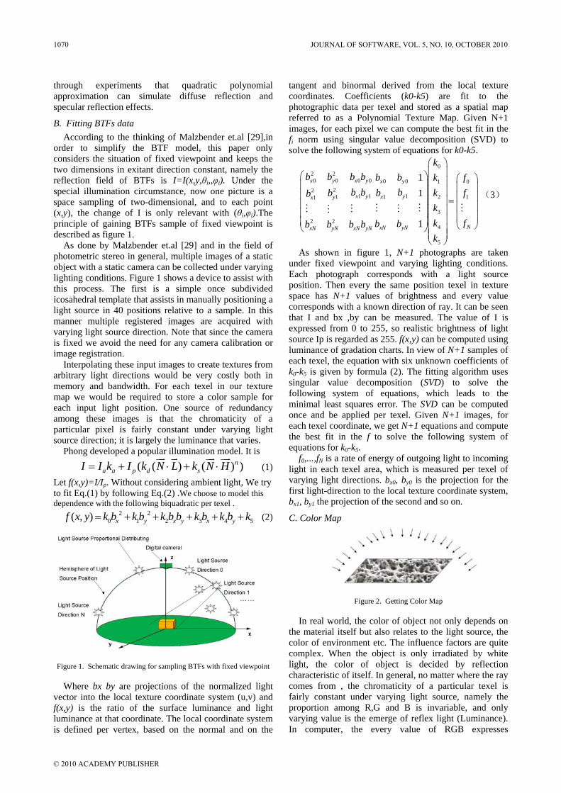
through experiments that quadratic polynomial approximation can simulate diffuse reflection and specular reflection effects.

B. Fitting BTFs data According to the thinking of Malzbender et.al [29],in

order to simplify the BTF model, this paper only considers the situation of fixed viewpoint and keeps the two dimensions in exitant direction constant, namely the reflection field of BTFs is I=I(x,y,θi,,φi). Under the special illumination circumstance, now one picture is a space sampling of two-dimensional, and to each point (x,y), the change of I is only relevant with (θi,φi).The principle of gaining BTFs sample of fixed viewpoint is described as figure 1.

As done by Malzbender et.al [29] and in the field of photometric stereo in general, multiple images of a static object with a static camera can be collected under varying lighting conditions. Figure 1 shows a device to assist with this process. The first is a simple once subdivided icosahedral template that assists in manually positioning a light source in 40 positions relative to a sample. In this manner multiple registered images are acquired with varying light source direction. Note that since the camera is fixed we avoid the need for any camera calibration or image registration.

Interpolating these input images to create textures from arbitrary light directions would be very costly both in memory and bandwidth. For each texel in our texture map we would be required to store a color sample for each input light position. One source of redundancy among these images is that the chromaticity of a particular pixel is fairly constant under varying light source direction; it is largely the luminance that varies.

Phong developed a popular illumination model. It is

( ( ) ( ) )na a p d sI I k I k N L k N H= + ⋅ + ⋅

uur ur uur uur (1)

Let f(x,y)=I/Ip. Without considering ambient light, We try to fit Eq.(1) by following Eq.(2) .We choose to model this dependence with the following biquadratic per texel .

2 20 1 2 3 4 5( , ) x y x y x yf x y k b k b k b b k b k b k= + + + + + (2)

Figure 1. Schematic drawing for sampling BTFs with fixed viewpoint

Where bx by are projections of the normalized light vector into the local texture coordinate system (u,v) and f(x,y) is the ratio of the surface luminance and light luminance at that coordinate. The local coordinate system is defined per vertex, based on the normal and on the

tangent and binormal derived from the local texture coordinates. Coefficients (k0-k5) are fit to the photographic data per texel and stored as a spatial map referred to as a Polynomial Texture Map. Given N+1 images, for each pixel we can compute the best fit in the fi norm using singular value decomposition (SVD) to solve the following system of equations for k0-k5.

02 20 0 0 0 0 0 1 0

221 1 1 211 11

32 2

4

5

11

1

x y x y x y

x y yxyx

NxN yNxN yN xN yN

kb b b b b b k f

b b b kbb fbk

fkb bb b b bk

⎛ ⎞⎜ ⎟⎛ ⎞ ⎛ ⎞⎜ ⎟⎜ ⎟ ⎜ ⎟⎜ ⎟⎜ ⎟ ⎜ ⎟=⎜ ⎟⎜ ⎟ ⎜ ⎟⎜ ⎟⎜ ⎟ ⎜ ⎟⎜ ⎟⎜ ⎟ ⎝ ⎠⎝ ⎠⎜ ⎟⎜ ⎟⎝ ⎠

M MMM MM M

（3）

As shown in figure 1, N+1 photographs are taken under fixed viewpoint and varying lighting conditions. Each photograph corresponds with a light source position. Then every the same position texel in texture space has N+1 values of brightness and every value corresponds with a known direction of ray. It can be seen that I and bx ,by can be measured. The value of I is expressed from 0 to 255, so realistic brightness of light source Ip is regarded as 255. f(x,y) can be computed using luminance of gradation charts. In view of N+1 samples of each texel, the equation with six unknown coefficients of k0-k5 is given by formula (2). The fitting algorithm uses singular value decomposition (SVD) to solve the following system of equations, which leads to the minimal least squares error. The SVD can be computed once and be applied per texel. Given N+1 images, for each texel coordinate, we get N+1 equations and compute the best fit in the f to solve the following system of equations for k0-k5.

f0,...,fN is a rate of energy of outgoing light to incoming light in each texel area, which is measured per texel of varying light directions. bx0, by0 is the projection for the first light-direction to the local texture coordinate system, bx1, by1 the projection of the second and so on.

C. Color Map

Figure 2. Getting Color Map

In real world, the color of object not only depends on the material itself but also relates to the light source, the color of environment etc. The influence factors are quite complex. When the object is only irradiated by white light, the color of object is decided by reflection characteristic of itself. In general, no matter where the ray comes from , the chromaticity of a particular texel is fairly constant under varying light source, namely the proportion among R,G and B is invariable, and only varying value is the emerge of reflex light (Luminance). In computer, the every value of RGB expresses



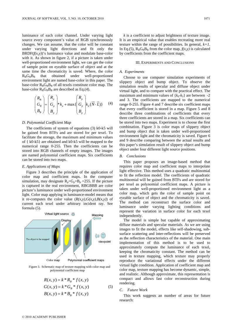
luminance of each color channel. Under varying light source every component’s value of RGB synchronously changes. We can assume, that the color will be constant under varying light directions and fit only the BRDF(f(x,y))’s luminance value and modulate base-color with it. As shown in figure 2, if a picture is taken under well-proportioned environment light, we can get the color of sample point on eyeable surface of object and at the same time the chromaticity is saved. Where, the color RBGBBB that obtained under well-proportioned environment light are named base-color in this paper. The base-color RBGBBB of all texels constitute color map. The base-color RBGBBB are described as Eq.(4).

* max ( )p pB

B p a p d

B p p

R RRG G k G k N LB B B

⎛ ⎞ ⎛ ⎞⎛ ⎞⎜ ⎟ ⎜ ⎟⎜ ⎟ = + ⋅⎜ ⎟ ⎜ ⎟⎜ ⎟⎜ ⎟ ⎜ ⎟⎜ ⎟

⎝ ⎠ ⎝ ⎠ ⎝ ⎠

uur ur (4)

D. Polynomial Coefficient Map The coefficients of system of equations (3) k0-k5 will

be gained from BTFs and are stored for per texel. To facilitate the storage, the maximum and minimum values of k0-k5 are obtained and k0-k5 will be mapped to the numerical range 0-255. Then the coefficients can be stored into RGB channels of empty images. The images are named polynomial coefficient maps. Six coefficients can be stored into two maps.

E. Applications of Maps Figure 3 describes the principle of the application of

color map and coefficient maps. In the computer simulation, may designate Rp=Gp=Bp =255. If the picture is captured in the real environment, RBGBBB are color picture’s luminance under well-proportioned environment light. Color map applying in luminance-model means that it re-computes the color value (R(x,y),G(x,y),B(x,y)) of current each texel under arbitrary incident ray. See formula (5).

Figure 3. Schematic map of texture mapping with color map and

polynomial coefficient map

( , ) * * ( , )( , ) * * ( , )( , ) * * ( , )

B

B

B

R x y k R f x yG x y k G f x yB x y k B f x y

===

(5)

k is a coefficient to adjust brightness of texture image. It is an empirical value that enables recreating more real texture within the range of possibilities. In general, k=1. In Eq.(5), RBGBBB from the color map, f(x,y) is calculated by coefficients from the coefficient maps.

III. EXPERIMENTS AND CONCLUSIONS

A. Experiments Choose to use computer simulation experiments of

slippery object and bump object. To observe the simulation results of specular and diffuse object under virtual light, and to compare with the practical effect. The maximum and minimum values of k0-k5 are between -2 and 3. The coefficients are mapped to the numerical range 0-255. Figure 4 and 7 describe six coefficient maps that every coefficient is stored in a map. Figure 5 and 8 describe three combinations of coefficients that every three coefficients are stored in a map. Six coefficients can be stored into two maps. Experiment is to choose the first combination. Figure 3 is color maps of slippery object and bump object that is taken under well-proportioned environment light and the chromaticity is saved. Figure 6 and 9 describe comparing between the actual results and this paper’s simulation result of slippery object and bump object under four different light source positions.

B. Conclusions This paper proposes an image-based method that

requires color map and coefficient maps to interpolate light effective. This method uses a quadratic multinomial to fit the reflection model. The coefficients of quadratic multinomial will be gained from BTFs and are stored for per texel as polynomial coefficient maps. A picture is taken under well-proportioned environment light as a color map, which gets the color of sample point on eyeable surface of object and the chromaticity is saved. The method can reconstruct the surface color and luminance under varying lighting conditions and represent the variation in surface color for each texel independently.

The model is simple but capable of approximating diffuse materials and specular materials. As we are using images to fit the model, effects like self-shadowing, sub-surface scattering and inter-reflections will be preserved as the reflection characteristics of the material. One main implementation of this method is to be used to approximately compute the luminance of each texel, keeping the chromaticity constant. The method can be used in texture mapping, which texture may properly reproduce the variational effects under the different virtual light condition. Application of coefficient map and color map, texture mapping has become dynamic, simple, and realistic. Although approximate, this representation is compact and allows fast color reconstruction during rendering.

C. Future Work This work suggests an number of areas for future

research:



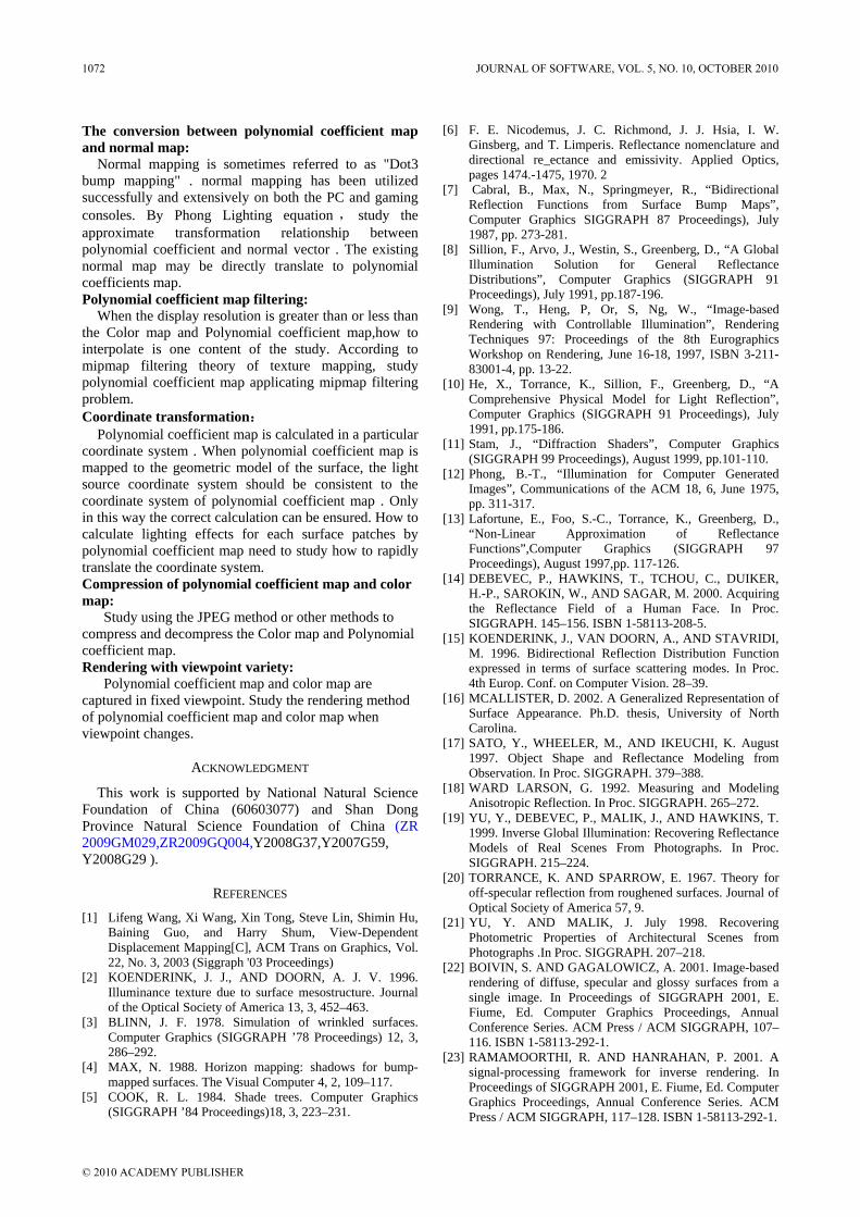
The conversion between polynomial coefficient map and normal map:

Normal mapping is sometimes referred to as "Dot3 bump mapping" . normal mapping has been utilized successfully and extensively on both the PC and gaming consoles. By Phong Lighting equation ， study the approximate transformation relationship between polynomial coefficient and normal vector . The existing normal map may be directly translate to polynomial coefficients map. Polynomial coefficient map filtering:

When the display resolution is greater than or less than the Color map and Polynomial coefficient map,how to interpolate is one content of the study. According to mipmap filtering theory of texture mapping, study polynomial coefficient map applicating mipmap filtering problem. Coordinate transformation：

Polynomial coefficient map is calculated in a particular coordinate system . When polynomial coefficient map is mapped to the geometric model of the surface, the light source coordinate system should be consistent to the coordinate system of polynomial coefficient map . Only in this way the correct calculation can be ensured. How to calculate lighting effects for each surface patches by polynomial coefficient map need to study how to rapidly translate the coordinate system. Compression of polynomial coefficient map and color map:

Study using the JPEG method or other methods to compress and decompress the Color map and Polynomial coefficient map. Rendering with viewpoint variety:

Polynomial coefficient map and color map are captured in fixed viewpoint. Study the rendering method of polynomial coefficient map and color map when viewpoint changes.

ACKNOWLEDGMENT

This work is supported by National Natural Science Foundation of China (60603077) and Shan Dong Province Natural Science Foundation of China (ZR 2009GM029,ZR2009GQ004,Y2008G37,Y2007G59, Y2008G29 ).

REFERENCES

[1] Lifeng Wang, Xi Wang, Xin Tong, Steve Lin, Shimin Hu, Baining Guo, and Harry Shum, View-Dependent Displacement Mapping[C], ACM Trans on Graphics, Vol. 22, No. 3, 2003 (Siggraph '03 Proceedings)

[2] KOENDERINK, J. J., AND DOORN, A. J. V. 1996. Illuminance texture due to surface mesostructure. Journal of the Optical Society of America 13, 3, 452–463.

[3] BLINN, J. F. 1978. Simulation of wrinkled surfaces. Computer Graphics (SIGGRAPH ’78 Proceedings) 12, 3, 286–292.

[4] MAX, N. 1988. Horizon mapping: shadows for bump-mapped surfaces. The Visual Computer 4, 2, 109–117.

[5] COOK, R. L. 1984. Shade trees. Computer Graphics (SIGGRAPH ’84 Proceedings)18, 3, 223–231.

[6] F. E. Nicodemus, J. C. Richmond, J. J. Hsia, I. W. Ginsberg, and T. Limperis. Reflectance nomenclature and directional re_ectance and emissivity. Applied Optics, pages 1474.-1475, 1970. 2

[7] Cabral, B., Max, N., Springmeyer, R., “Bidirectional Reflection Functions from Surface Bump Maps”, Computer Graphics SIGGRAPH 87 Proceedings), July 1987, pp. 273-281.

[8] Sillion, F., Arvo, J., Westin, S., Greenberg, D., “A Global Illumination Solution for General Reflectance Distributions”, Computer Graphics (SIGGRAPH 91 Proceedings), July 1991, pp.187-196.

[9] Wong, T., Heng, P, Or, S, Ng, W., “Image-based Rendering with Controllable Illumination”, Rendering Techniques 97: Proceedings of the 8th Eurographics Workshop on Rendering, June 16-18, 1997, ISBN 3-211-83001-4, pp. 13-22.

[10] He, X., Torrance, K., Sillion, F., Greenberg, D., “A Comprehensive Physical Model for Light Reflection”, Computer Graphics (SIGGRAPH 91 Proceedings), July 1991, pp.175-186.

[11] Stam, J., “Diffraction Shaders”, Computer Graphics (SIGGRAPH 99 Proceedings), August 1999, pp.101-110.

[12] Phong, B.-T., “Illumination for Computer Generated Images”, Communications of the ACM 18, 6, June 1975, pp. 311-317.

[13] Lafortune, E., Foo, S.-C., Torrance, K., Greenberg, D., “Non-Linear Approximation of Reflectance Functions”,Computer Graphics (SIGGRAPH 97 Proceedings), August 1997,pp. 117-126.

[14] DEBEVEC, P., HAWKINS, T., TCHOU, C., DUIKER, H.-P., SAROKIN, W., AND SAGAR, M. 2000. Acquiring the Reflectance Field of a Human Face. In Proc. SIGGRAPH. 145–156. ISBN 1-58113-208-5.

[15] KOENDERINK, J., VAN DOORN, A., AND STAVRIDI, M. 1996. Bidirectional Reflection Distribution Function expressed in terms of surface scattering modes. In Proc. 4th Europ. Conf. on Computer Vision. 28–39.

[16] MCALLISTER, D. 2002. A Generalized Representation of Surface Appearance. Ph.D. thesis, University of North Carolina.

[17] SATO, Y., WHEELER, M., AND IKEUCHI, K. August 1997. Object Shape and Reflectance Modeling from Observation. In Proc. SIGGRAPH. 379–388.

[18] WARD LARSON, G. 1992. Measuring and Modeling Anisotropic Reflection. In Proc. SIGGRAPH. 265–272.

[19] YU, Y., DEBEVEC, P., MALIK, J., AND HAWKINS, T. 1999. Inverse Global Illumination: Recovering Reflectance Models of Real Scenes From Photographs. In Proc. SIGGRAPH. 215–224.

[20] TORRANCE, K. AND SPARROW, E. 1967. Theory for off-specular reflection from roughened surfaces. Journal of Optical Society of America 57, 9.

[21] YU, Y. AND MALIK, J. July 1998. Recovering Photometric Properties of Architectural Scenes from Photographs .In Proc. SIGGRAPH. 207–218.

[22] BOIVIN, S. AND GAGALOWICZ, A. 2001. Image-based rendering of diffuse, specular and glossy surfaces from a single image. In Proceedings of SIGGRAPH 2001, E. Fiume, Ed. Computer Graphics Proceedings, Annual Conference Series. ACM Press / ACM SIGGRAPH, 107–116. ISBN 1-58113-292-1.

[23] RAMAMOORTHI, R. AND HANRAHAN, P. 2001. A signal-processing framework for inverse rendering. In Proceedings of SIGGRAPH 2001, E. Fiume, Ed. Computer Graphics Proceedings, Annual Conference Series. ACM Press / ACM SIGGRAPH, 117–128. ISBN 1-58113-292-1.



[24] GIBSON, S., HOWARD, T., AND HUBBOLD, R. 2001. Flexible image-based photometric reconstruction using virtual light sources. Computer Graphics Forum 20, 3. ISSN 1067-7055.

[25] WESTIN, S., ARVO, J., AND TORRANCE, K. 1992. Predicting Reflectance Functions From Complex Surfaces. In Proc. SIGGRAPH. 255–264.

[26] LU, R., KOENDERINK, J., AND KAPPERS, A. 1998. Optical Properties (bidirectional reflectance distribution functions) of velvet. Applied Optics 37, 25 (Sept.), 5974–5984.

[27] MARSCHNER, S. 1998. Inverse rendering for computer graphics. Ph.D. thesis, Cornell University.

[28] S. E. Chen. Quicktime vr: An image-based approach to virtual environment navigation. In SIGGRAPH 1995, pages 29–38.

[29] T. Malzbender, D. Gelb, and H. Wolters. Polynomial texture maps. In SIGGRAPH 2001, pages 519–528.

[30] W.-C. Chen, J.-Y. Bouguet, M. H. Chu, and R. Grzeszczuk. Light field mapping: Efficient representation and hardware rendering of surface light fields. In SIGGRAPH 2002, pages 447–456.

[31] DEBEVEC, P., TAYLOR, C., AND MALIK, J. 1996. Modeling and rendering architecture from photographs: A hybrid geometry- and image-based approach. In Proc. SIGGRAPH. 11–20.

[32] GORTLER, S., GRZESZCZUK, R., SZELINSKI, R., AND COHEN, M. 1996. The Lumigraph. In Proc. SIGGRAPH. 43–54.

[33] LEVOY, M. AND HANRAHAN, P. 1996. Light Field Rendering. In Proc. SIGGRAPH. 31–42.

[34] WOOD, D., AZUMA, D., ALDINGER, K., CURLESS, B., DUCHAMP, T., SALESIN, D., AND STUETZLE, W. 2000. Surface Light Fields for 3D Photography. In Proc. SIGGRAPH. 287–296.

[35] MILLER, G., RUBIN, S., AND PONCELEON, D. 1998. Lazy decompression of surface light fields for precomputed global illumination. In 9th Eurographics Workshop on Rendering. 281–292.

[36] T. Malzbender, D. Gelb, and H. Wolters. Polynomial texture maps. In SIGGRAPH 2001, pages 519–528.

[37] K. J. Dana, B. van Ginneken, S. K. Nayar, and J. J. Koenderink. Reflectance and texture of real-world surfaces. ACM TOG, 18(1):1–34, 1999.

[38] Gregory J. Ward. Measuring and modeling anisotropic reflection. In Proceedings of the 19th annual conference on Computer graphics and interactive techniques, pages 265–272. ACM Press, 1992.

[39] Jan Kautz and Michael McCool. Interactive rendering with arbitrary BRDFs using separable approximations. In Tenth Eurographics Workshop on Rendering, pages 281–292, 1999.

[40] Ravi Ramamoorthi and Pat Hanrahan. Frequency space environment map rendering. In Proceedings of the 29th annual conference on Computer graphics and interactive techniques, pages 517–526. ACM Press, 2002.

[41] Peter-Pike Sloan, Jan Kautz, and John Snyder. Precomputed radiance transfer for real-time rendering in dynamic, low-frequency lighting environments. In Proceedings of the 29th annual conference on Computer graphics and interactive techniques, pages 527–536. ACM Press, 2002.

[42] Lutz Latta and Andreas Kolb. Homomorphic factorization of BRDF-based lighting computation. In Proceedings of

the 29th annual conference on Computer graphics and interactive techniques, pages 509–516. ACM Press, 2002.

[43] Tom Malzbender, Dan Gelb, and Hans Wolters. Polynomial texture maps. In Proceedings of the 28th annual conference on Computer graphics and interactive techniques, pages 519–528. ACM Press, 2001.

[44] Huijian Han, Caiming Zhang, Jiaye Wang, Projections-based Rendering Arbitrary Lighting Effects, Journal of Computational Information System, pages 411–416.2007；.

Huijian Han, Male, was born in

HeZe city, China, in December 19, 1971. In 2000, Han is a master majoring in Computer Software Theory and Techniques of Shandong University, China, and now as Computer Applied Technique Ph. D. candidate in Shandong University. Han’s major field of study is texture mapping of CG.

He is a PROFESSOR, MASTER TUTOR in School of Computer

Science & Technology of ShanDong Economic University and Shandong Prov. Key Lab of Digital Media Technology, in Jinan city, China. He participated in the work in 1992 and has long been engaged in computer technology in teaching and research work. He has published more than 30 papers in academic journals at home and abroad and participated in the preparation of two books. For example: Computer Graphics (Beijing, China: Science Press,2005); Concise Guide to Computer Graphics (Beijing, China, Higher Education Press,2007); Determining Knots by Minimizing Energy(Beijing , China, Journal of Computer Science and Technology, 2006). His current research interests include CG&CAGD, computer simulation and digital media techniques.

Prof. Han is a member of Chinese Association for System Simulation, Computer Society of Shandong Province, and Academic Committee of Shandong Prov. Key Lab of Digital Media Technology. Prof. Han received third prize of Shandong Province Natural Science Award in 2005, received first prize of Science and Technology Progress Award of People's Republic of China Ministry of Education in 2007 and received Outstanding Contribution Award from the Shandong Provincial Science and Technology Association in 2008.

Caiming Zhang, doctor,

professor of Computer Science and technical Department of Shandong Economic University, doctor tutor, president of computer applied technical institute. He has been devoted to digital media, GAGD, CG, science computer visualization, and so on. From 1991 to 1995, he made an academic visit to Tokyo Industrial University and studied for

the doctor degree there, and his research field is GAGD, Graphics, and image processing. From 1997 to 1999, he made an academic visit to Kentucky University and did research on the car exterior designing for Ford Motor Corp. as a postdoctoral.

.



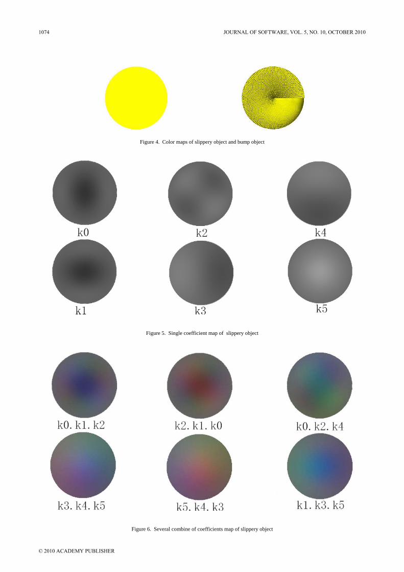
Figure 4. Color maps of slippery object and bump object

Figure 5. Single coefficient map of slippery object

Figure 6. Several combine of coefficients map of slippery object



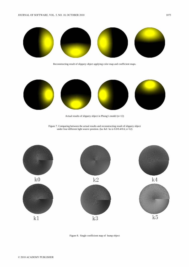
Reconstructing result of slippery object applying color map and coefficient maps.

Actual results of slippery object in Phong’s model (n=12)

Figure 7. Comparing between the actual results and reconstructing result of slippery object under four different light source position. (ka /kd / ks is 0.0/0.4/0.6; n=12)

Figure 8. Single coefficient map of bump object



Figure 9. Several combine of coefficients map of bump object

Reconstructing result of bump object applying color map and coefficient maps.

Actual results of bump object in Phong’s model

Figure 10. Comparing between the actual results and reconstructing result of bump object under four different light source position.



A Study on Framework and Realizing Mechanism of ISEE Based on Product Line

Jianli Dong

HuaiHai Institute of Technology / School of Computer Engineering, Lianyungang, 222005, China Email: [email protected]

Ningguo Shi

Lanzhou Resources & Environment Voc-Tech College/President Office, Lanzhou, 730021, China Email: [email protected]

Abstract—Using product line automatic production procedure and the management system of modern manufacturing industry for reference, a new model of integrated software engineering environment based on product line is put forward, and framework and realizing mechanism of the new model is mainly analyzed in this paper. The new model takes product line core asset (resource) components as the agent bus. The upper of it supports the product line development environment realizing the assembling production of software products, while the lower is traditional common software development environment implementing the development of source codes and documents of product line core resource components. Compared with the present available product line development environment models, the developing and realizing ability of the new one is completely similar to production mode of automatic product line and management system of current manufacturing industry, will be likely to become an ideal software production environment that the future software engineering industry develops. Index Terms—software product line, core assets, ISEE-integrated software engineering environment, software architecture, software component

I. INTRODUCTION

In recent years, with the gradual mature and application of the new techniques such as software architecture, software components, software large granularity reuse etc., software engineering method based on product line have aroused broad attention of software engineering filed and already become the hot spot and priority of the current studies in software engineering field. The core of software product line studies is to apply the techniques of software architecture, software components, software large granularity reuse and realize the industrialization and automatic production of mass custom-made software products in a specific field, which is similar to product line automatic production modes of modern manufacturing industry products (such as cars , TVs etc.). This is the ideal software production mode pursued for 40 years of software engineering development, which has the very important effect on the formation and development of modern software estate, and will produce the gigantic society and economic effect[1-3].

II. THE CURRENT SITUATION OF SOFTWARE PRODUCT LINE STUDIES

Owing to software engineering method based on product line there has been the fundamental change in software development from the traditional one-time, manual programming way, "algorithm + data structure + manpower code", into the industrialized production mode, " software architecture + software components +product line assembly (systematic reuse)", which is characterized by the production system of modern manufacturing industry (such as cars, TV sets etc.) Software product line approach must rely on the achievement of integrated development environment based on product line with the features of product line engineering and the production capacity. Such environment is called integrated software engineering environment based on product line Therefore, the research, realization and application of the integrated software engineering environment based on product line, play a very important role on the automation of software production and the industrialization of the software industry, has become strategic initiatives for the world to occupy the field of information industry, and promote rapid and sustainable economic and social development.

However, we should see clearly that the formation and development of the software product line engineering approach has used product line automatic production mode of modern manufacturing industry for reference based on engineering domain, software architecture, software components and software reuse technology. Its objective is to establish software product line and realize the industrialized production of software products by using the technologies of software architecture of specific field and system-level reuse of large granularity. Obviously, the integrated software engineering environment based on product line is essentially different from the current common software development environment which is structure-based or object-oriented software engineering approach (called the traditional development environment for short). The former is to realize the industrialization and automatic production of mass custom-made software products in a specific field in accordance with "software Architecture + components + assembly" of a specific field, While the latter is in accordance with "data structure + procedures + manual



encoding" meaning the development of one-time, from scratch software programs, and the general environment also determines the applicable extent of environment, modes of production, productivity and update transformation will be subject to many limitations. Moreover, it is fully different from the production mode and development direction of modern manufacturing industry, as a common product line can not be used to manufacture cars, airplanes, television and other products in different fields.

It is a pity that in the current process of research and development of integrated software development environment based on product line, people haven’t recognized the essential difference between traditional software development environment and modern integrated one. The studies and development of product line software engineering methodologies and integrated development environment is still carried out according to the traditional software engineering methods and ideas, which is not correct. As the CMU / SEI and a number of literature [4-5] have pointed out: so far, there is not the true sense of the integrated software engineering environment based on product line. In other words, the actual status of research and development is that a number of software companies introduce some concepts of components on the basis of its existing software development environment and add the appropriate number of controls, then think that it is transformed into the so-called integrated software engineering environment based on product line. For example, IBM's Rational, SUN's J2EE development environment, etc., are of this type, they are far below the true sense of automated assembly line with production capacity and features of software product line integrated development environment of modern manufacturing industry. Of course, for the interests of enterprises and several decades of software engineering development models, especially the system software and tools for software development process, it is natural and understandable, because enterprises have to take into account their existing products and interests. It is impossible to completely discard the existing large-scale and widely used software products, regardless of the risk to pursue a new product despite the wide range of applications with great prospects and economic benefits.

The paper focuses on a real sense of the software product line development environment model with product line production mode and capacity of modern manufacturing industry, and mainly studies its architecture and the realization of mechanism.

III. SOFTWARE ENGINEERING PROCESS AND LIFE-CYCLE MODEL BASED ON PRODUCT LINE

Essentially, software engineering environment based on product line is a kind of product line which similar to the automatic production line of modern manufacturing industry. It is also a new software engineering method and process to carry out mass customization production of software products in specific domain based on standard component of core resources such as software

architecture, component, connecting piece, production plan, specification, constraint, documents and so on. Therefore, what the most important for research on the product line software development environment is to set up software development process model and life-cycle model which suitable for the characteristics and the production methods of product line. It is used to describe the whole process of products development based on product line systematically, and then take this as a guide to determine the message-based application, tool configuration and production process.

Its goal is to describe the sequence of activities, workflow, the task framework, product submission and standards of software engineering process based on product line completely, clearly and specifically. And the guidelines to action and behavioral norms to implement the software product line engineering and software products would be the prerequisite and an important foundation for the research on the integrated software development environment. In recent years, there have been some preliminary research results on the research of product line engineering process model. For example: software product line double life cycle model and SEI model[7-8]. But there simple models can hardly meet the requirement of the whole process expressing ability of modern software management system, mode of producing, evolution of e-Learning, quality control and so on, such as the Multi-level upper and lower layer organization and management system of international, national, industry, domains and application and so on which owned by product line project, the engineering process characteristics and mode of multi-level iterative production methods and the evolution of multi-dimensional product.[13].

On the research and creation of the product line engineering process models and life-cycle, we firstly propose a kind of opened "N-life cycle model" suitable for software engineer based on product line. This model contain the whole process of product line software engineer, each operational phase division of inter process ,the customization of task framework, product quality standards, the entire process of monitoring the completion steps, management and technical characteristics completely. Compared with product line double life cycle model, SEI model and so on, N-life-cycle model, an open process model, which use for reference of the modern industry process and management system and has been proved to be more features and manage spatial of modern industry, meet the product line software project process modeling and expression ability[14].

IV. A NEW ISEE-MODEL BASED ON THE PRODUCT LINE CORE ASSET AND AGENT COMPONENTS BUS

With the research and development of software engineering methodology, the study of integrated software engineering environment has become very active in the field of software engineering. Integrated software engineering environment model is the foundation and prerequisite for integrated software engineering



environment .The research purpose is to create the environmental framework and its implementation mechanism, technologies and methods adapted for specific software engineering methods and the development process (life cycle). Now the integrated reference model generally accepted by software engineering field is the three-dimensional integrated model of web-based distributed computing environment proposed by NIST / ECMA, that is, three-dimensional integration of interface, tools and data [9]. However, the research and development of integrated software engineering environment based on the NIST / ECMA model are about the realization of a common software development environment and one-time, from scratch software product development process which is almost all limited to the traditional software engineering methodology. The ability of such an environment model, "Architecture + component + pipeline assembly", can not satisfy the software production environment and development model based on product line, which is the main basis for almost the blank about CMU /SEI’s evaluation of software product line development environment.

Integrated software engineering environment model based on product line not only has low-level and source code-level program development capabilities of traditional software engineering environment, but also the basic characteristics such as “ field, abstraction, publicity, and scalability, reusability and variability," owned by core resources (the system architecture and components, etc.) included in product line development environment and automated assembly capacity of system-level components characterized by mass custom-made production of product line. This is the nature difference between traditional software development environment and product line development environment, and also the key of the establishment of product line integrated development model.

The research and establishment of product line integrated software engineering environment model must be based on a correct and complete software product line engineering process model and a life-cycle model. Because product line software engineering process and the life cycle model is used to define and describe the production process and demands in the process of software development such as activities sequence, tasks framework, technical methods, management measures, submitted products quality, which is regarded as the guideline and norm of the implementation of software product line engineering and the production of software products, and become the important foundation and the prerequisite for studies of integrated software engineering environment based on product line.

In the current studies of product line engineering process model, there have been some preliminary research results, for instance, the most representative of process models are the dual life cycle model of software product line and SEI (CMU / SEI) model [10-12] However, these simple models are difficult to express

and describe the management system, production mode, the evolution of the process, quality control and other features and capacity needs that software product line engineering environment should have, such as international and domestic, industries and enterprises multi-level organization and management system of product line, multi-level iterative production mode and multi-stage products evolution mode. Through the research, in the literature [13-14] an open "N-Life Cycle Model," possessing automatic production features and management mechanism of modern manufacturing industry is proposed, and based on this model, product line integrated software engineering environment model is designed and established.(shown in Figure 1).

As figure 1 shows, product line software engineering environment model is an open and multi-level architecture new model of software engineering environment based on the conceptual model of unified product line engineering, the data model of granularity and reuse of core assets, the behavioral model of components assembly production, the evolution model of the iteration between core assets development and software products manufacture.

The architecture of this new model is essentially a double-environment model taking the core assets component as the bus, the upper is integrated software development environment based on product line supporting software products’ automatic assembly production of product line, while the lower is the traditional software development environment based on traditional software engineering methods supporting the development of core assets components’ source code and common programs. It is obvious that this new model of integrated environment also includes software production environment and production mode similar to automatic assembly production mode and management mechanism of modern manufacturing industry. It is a real sense of the integrated software engineering environment based on product line.

Figure 1 Note: Filled boxes represent the products of the process or tools or phases. No filled boxes represent the process or tools.

Product Line Interface Integration and Interface Services (interface layer): AT- Analysis Tools Interface, DT-Design Tools Interface, AST-ASsembly Tools Interface.

Standard Engineering Tools: PLSC-Product Line Standard Classification, PLSD-Product Line Standard Design, PLSR-Product Line Standard Release; DA-Domain Analysis Standard, DD-Domain Design Standard, DI-Domain Implementing Standard.

Domain Engineering Tools: DA-Domain Analysis, DD-Domain Design, DI-Domain Implementation

Application Engineering Tools: AA-Application Analysis, AD-Application Design, AI-Application Implementation.

Core Assets Database Platform and Data Integration Services: NSC-National Standard Components, ISC-Industry Standard Components, ESC-Enterprise Standard Components, LAC-Local Agent Components.



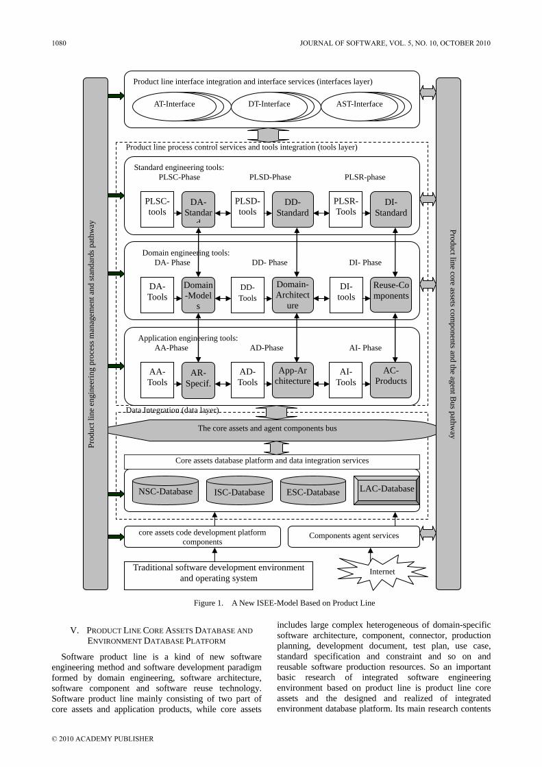
V. PRODUCT LINE CORE ASSETS DATABASE AND ENVIRONMENT DATABASE PLATFORM

Software product line is a kind of new software engineering method and software development paradigm formed by domain engineering, software architecture, software component and software reuse technology. Software product line mainly consisting of two part of core assets and application products, while core assets

includes large complex heterogeneous of domain-specific software architecture, component, connector, production planning, development document, test plan, use case, standard specification and constraint and so on and reusable software production resources. So an important basic research of integrated software engineering environment based on product line is product line core assets and the designed and realized of integrated environment database platform. Its main research contents

Figure 1. A New ISEE-Model Based on Product Line

NSC-Database ISC-Database ESC-Database

The core assets and agent components bus

Product line core assets components and the agent B

us pathway

Prod

uct l

ine

engi

neer

ing

proc

ess m

anag

emen

t and

stan

dard

s pat

hway

Traditional software development environment and operating system

core assets code development platform components

Components agent services

Internet

Domain engineering tools: DA- Phase DD- Phase DI- Phase

DA- Tools

Domain-Model

s

DD- Tools

Domain-Architect

ure

DI- tools

Reuse-Components

Application engineering tools: AA-Phase AD-Phase AI- Phase

AA- Tools

AR- Specif.

AD- Tools

App-Ar chitecture

AI- Tools

AC- Products

Product line interface integration and interface services (interfaces layer)

Product line process control services and tools integration (tools layer)

AT-Interface DT-Interface AST-Interface

Data Integration (data layer)

Standard engineering tools: PLSC-Phase PLSD-Phase PLSR-phase

DA- Standar

d

PLSC- tools

PLSD-tools

DD- Standard

PLSR-Tools

DI- Standard

Core assets database platform and data integration services

LAC-Database



includes: the study of the data model possess of the ability of core resource data expression and description, product line core assets database schema design, the research of operation mechanism and management ability on product line core assets storage, classification, retrieval, query, version, reuse and optimization and so on. That is, in the demand of capacity, except having the conventional database storage and management capabilities, core assets database should provide rich and reused production resource and convenient resource retrieval, query, reuse, assembly and configuration and so on and management ability for software products customization, assembly and production, this is also the basic goal of the research on product line core assets and environment database system.[15-16]

Currently, the most common and extensive database model is relational data model in the design of product line complex heterogeneous core resource database model, but for the capability defect of relation model such as poor expression ability and semantic fault, the establish of product line core assets database model must adopt object-oriented model that having ultra-intense expression ability and good mechanism, to complete the expression of complex heterogeneous resource data and the demand of modeling; in the design of core assets database, research and establish the multi-view core resource database mode which either has the features of three layer structure of product line architecture style, architecture framework and architecture component or mapping view, reuse degree view and relational view, to realize product line engineering characters and management requirements database, here not only provide management function of core assets such as storage, classification, retrieval, version, optimization and configuration, it also provide good mechanism and methods of data integration, tool integration and interface integration. Furthermore, to consider current network running environment, core assets database platform should offer Internet proxy function to realize localization and network of component integration. These are the basic characteristics and ability that environment database system must have.

VI. THE REALIZING MECHANISM OF PRODUCT LINE INTEGRATED DEVELOPMENT ENVIRONMENT

Here it must be pointed out that as shown in Figure 1, the nature difference between the integrated software engineering environment model based on product line containing software development environment and traditional sense of the software (program) development environment is levels of architecture. The architecture of this new model is essentially a double-environment taking the core assets component as the bus, the upper is product line software engineering environment realizing high-level, system-level software products’ automated assembly production; while the lower is traditional software development environment realizing low-level, source-level components of product line development.

In the process of the study and realization of software engineering environment model, the standard reference model accepted by the industry is three-dimensional

integrated model and the realizing mechanism proposed by NIST / ECMA. In this model, the integrated software engineering environment consists of three aspects of data information including environment interface, environment tools and environment data, which is in accordance with the hierarchical structure of information from top to bottom known as interface layer, tools layer and data layer. Interface layer implements interface integration and management, whose function is receiving user’s information and requests, and also dealing with tools call and the returning result data. Tools Layer carries out the integration and management of tools, whose upper part provides services for interface layer and lower part fulfills data access and sharing. Data layer is actually environment database platform realizing the integration, storage and management of the environmental data (resources).

In fact, the realizing mechanism and methods given by NIST / ECMA model is in line with people’s day-to-day development, use and operation of computer. The common abstract model can be used for reference in any development and realization of software engineering environment. Only the interface, tools and data of the environment are of different.

As shown in Figure 1, in the study of the realizing mechanism of the integrated software engineering environment model based on product line, we still use the realizing mechanism and methods of NIST / ECMA widely accepted by the current software engineering industry, but interfaces in different environments, tools and data, as well as their behavior and ability demand change fundamentally. As far as the architecture of the new model is concerned, the realization of the integrated software engineering environment on the top of core resources component bus should be based on the provisions and requirements of product line engineering process models and life-cycle model and the management and development tools should be developed and deployed to meet all kinds of projects and internal tasks need at different stages, then the integration of interface, tools and data should be achieved as shown in figure 1 in accordance with the hierarchical structure from top to bottom known as interface layer, tools layer and data layer. [17-20]

Interface layer implements man-machine interface management, whose function is to receive user’s operation information and call requests, and also dealing with tools call and the returning result data according to software product line engineering process and production process. The integration of interface should include vertical product line standards, field and application etc. (in Figure 1) and other various projects, as well as the related development tools and resource data interface of different stages of lateral various projects’ internal analysis, design and realization etc.

Tools Layer carries out the integration and management of tools, whose upper part provides services for interface layer. In order to achieve tools integration shown in Figure 1, a complete understanding of tool layer standards and vertical iteration, the evolution and



constraints of domain and applied engineering of the integrated environment should be possessed, as well as the horizontal iteration, the evolution and constraints of different phases of various projects’ internal analysis, design and realization. Thus determines the demand for tools and call between tools, collaboration, communication and control interoperability.

As shown in figure 1, in accordance with product line development process and methods a variety of engineering tools are integrated in tool layer. Among them, the product line engineering should integrate: the standard classification tool of product line, the standard design tools and standard publishing tools etc. The domain engineering should integrate: the field of analysis modeling tools, domain architecture (style, framework and model, etc.) design tools, domain architecture and components implementation tools. Application engineering should integrate: application requirement analysis modeling tools, application architecture and components design tools, application production (components assembly, test analysis) tools, etc. As tool Layer it should ensure the realization of integrated engineering tools, at the same time, it is also necessary to achieve natural integration with data layer and interface layer. That is, tools integration not only ensures call, scheduling, communication, collaboration and interoperability, but also ensures that tools for data access and sharing, and provides users with comprehensive services.

The main function of data layer is realizing integration, storage and management of the environmental data. Data layer is composed of core assets component and the agent bus (including the agent component) as well as core assets component database platform. The component bus provides access interface for tools layer in accordance with a unified concept model and data model to implement tools layer’s integration on data layer and have access to the component database and carry out management operations. Component database in accordance with national, industry and enterprise standards is divided into three categories in order to meet production standards demand of different levels of software product line. According to product line engineering process and the characteristics of assembly production, a core resources component and the agent channel have been set up on the right of Figure 1, the main function is to provides a good access mechanism to components database for interface layer and tools layer. Such a mechanism ensures that assembly line production of software products (family) is automatic assembly process and industrial production mode taking standard components as parts. The components bus and the channel is just the conveyor belt to provide standard components. In this product line integrated environment, product line production of software products also means that it is a high-level, system-level software component assembly process, rather than traditional low-level development environment and code-level software programming process.

In the realizing mechanism of environment data integration, the design and the realization of the environment database platform need to be particularly emphasized. The product line core resources mainly includes a large number of complex heterogeneous data resources such as domain-specific software architecture, components, connectors, production plan, development documents, test plans and use cases, standards and constraints etc. Therefore, data model of complex heterogeneous resources, database model of core resources and the design and creation of core resources database platform will become the key to achieve environment data integration. In the design of database model, now the most widely used database model is a relational data model, However, due to defects in the ability of the relational model (such as poor expression, semantic faults, etc.), the design of product line core resources data model must be the object-oriented model with super-strong communication skills and a good control mechanism in order to complete the expression and modeling needs of complex heterogeneous resources data. The designed and created core resources database schema need to have not only product line architecture style, architecture framework, the three-tier organizational structure of architecture components, but also the multi-view core resource database schema including the map view, reuse view, and relational view in order to achieve the characteristics of product line engineering and the database capacity of management needs. For the realization of the core resources database support platform, both management capabilities such as the storage of core resources, classification, search, optimization, version and configuration etc. and the good mechanisms and methods including data integration, tool integration and interface integration need to be provided. [21-23]

In the data layer is the development platform for core assets code-level components and the traditional general software development environment, mainly used to support the development of the source code programs and documents of core resources components. Of course, as product line core resources components, the third-party components can be directly invoked (COTS: Commercial Off-The-Shell) in the software product Line. Therefore, it is necessary to introduce the agent mechanism of components to the local agents and components bus as a special delivery mechanism. The lowest part of the integrated environment is the network environment and the operating system, and it will not go into details here.

VII. CONCLUSION

In summary, for the realization of product line engineering environment this paper first propose a new product line integrated software engineering environment model whose architecture and realization method are totally different from traditional one based on the recent theories, techniques and methods such as software architecture, components, reuse, domain engineering etc. in order to achieve the industrialization and automatic production of software products. The architecture and the



realizing mechanism of integrated development environment based on product line are fully similar to the automatic product line environment and production mode of modern manufacturing industry reflecting a new idea of the research and development of integrated software engineering environment. It represents the forefront of the research and development of modern software engineering methodologies, and has the guiding significance for the formation and development of modern software industry.

Of course, we should clearly find that the studies, realization and applications of integrated software engineering environment based on the product line needed to be carried on compared with automated production line of modern manufacturing industry. We still need to persist and make tireless efforts to do some pioneering work for the early realization of industrialization and automatic production of software products.

ACKNOWLEDGMENT

This project is supported by Fund of Jiangsu University Natural Science Basic Research Project, Grant No. 08KJD520013.

REFERENCES

[1] YANG FuQing, “Thinking on the Development of Software Engineering Technology,” JOURNAL OF SOFTWARE, 2005, 16(1): 1-7.

[2] MEI Hong, SHEN Jun-Rong, “Progress of Research on Software Architecture,” JOURNAL OF SOFTWARE, 2006, 17(6): 1257-1275.

[3] Wang Zhijia, Fei YuKuai, Software Component Technology and Application, BeiJing: Science Press, 2005.4.

[4] Paol.Clements, Linda Nort-hrop, Software Product Lines: Practices and Patterns (SEI Series in Software Engineering), Addison Wesley/Pearson. 2003.

[5] Zhang YouSheng, Software Architecture (first edition), BeiJing: TSingHua University Press, 2004.1.

[6] Paol. Clements, Linda Nort-hrop(America, the Original Author), Zhang Li, Wang Lei(China, Translators), “Software Product Lines: Practices and Patterns”, Tsinghua University Press(Beijing), 2003.

[7] Samuel A. Ajila, Ali B. Kaba, “Evolution support mechanisms for software product line process”, Journal of Systems and Software, Vol81(10), pp.1784-1801,October 2008.

[8] Daniel Mellado, Eduardo Fernández-Medina, Mario Piattini, “Towards security requirements management for software product lines: A security domain requirements engineering process”, Computer Standards & Interfaces, Vol.30(6), pp.361-371, 2008.

[9] Minder Chen, Ronald J. Norman, "A framework for integrated CASE", IEEE Software, 9(2), 1992, 18-22.

[10] Zhang YouSheng. Software Architecture (second edition). BeiJing: TSingHua University Press, 2007.1

[11] Kang KC, “Issues in Component-Based Software Engineering[C/OL],” 99 International Workshop on Component Based Software Engineering, http://www.sei.cmu.edu/cbs/ icse99/ papers/ icse992papers. pdf, 1999, 207-212.

[12] Kwanwoo Lee, Kyo C Kang, Jaejoon Lee, “Concepts and Guidelines of Feature Modeling for Product Line Software Engineering,” In: Proc 7th Int’l Conf Software Reuse. London, UK: Springer-Verlag, LNCS2319,2002:62-77.

[13] Dong Jianli. “Research on software engineering process model based on software product line architecture”, Computer Engineering and Design, 2008,29(12):3016-3018.

[14] Dong Jianli, Jianzhou Wang. “The research of software product line engineering process and it’s integrated development environment model”, ISCSCT-2008 Proceeding, IEEE Computer Society, Vol.1, pp.66-71.

[15] Paul Brown, “Distributed component database management systems”, Component Database Systems, 2001, pp.29-70.

[16] IEEE, Inc. “Information Technology--Guideline for the Evaluation and Selection of CASE Tools (IEEE Std 1462-1988). New York, NY:IEEE Computer Society Press, 1998.

[17] P. Lempp, “Integrated computer support in the software engineering environment EPOS — Possibilities of support in system development projects,” Microprocessing and Microprogramming, Volume 18, Issues 1-5, December 1986, Pages 223-232.

[18] Ian Thomas & Brian A.Neijmeh, “Definitions of tool integration for environments,” IEEE Software, March, 1992.

[19] Brown, A.W. Carney, Ｄ.Ｊ., etc. “Principle of CASE tool integration,” Oxford, U.K.: Oxford University Press,1994.

[20] S Chen, J. M. Drake, W. T. Tsai, “Database requirements for a software engineering environment: criteria and empirical evaluation,” Information and Software Technology, Volume 35, Issue 3, March 1993, P149-161.

[21] M. P. Papazoglou, L. Marinos, “On integrating database modeling constructs for software engineering databases,” Microprocessing and Microprogramming, Volume 27, Issues 1-5, August 1989, P113-120.

[22] Andreas Geppert, Klaus R. Dittrich, “Component database systems: Introduction, foundations, and overview,” Component Database Systems, 2001, P1-28.

[23] Magnus Eriksson, Jürgen Börstler, Kjell Borg, “Managing requirements specifications for product lines – An approach and industry case study,” Journal of Systems and Software, Volume 82, Issue 3, March 2009, P435-447.

Jianli DONG was born in Shanxi province, China, in 1957. He got his Bachelor of Mathematics Science in, Northwest Normal University, Lanzhou, Gansu province, China, in 1988 and got his Master of Software Engineering in Beijing University of Aeronautics and Astronautics, Beijing, China, in 1995. He is now a professor at the School of Computer Engineering in HuaiHai Institute Technology, Lianyungang, China. He has published 40 papers, and completed many reseach projects, and won 6 times scientific and technological progress awards from the provance and military.

Mr. Dong current research interests include software engineering, integrated software engineering enviroment, software architecture, engineering database system, object-oriented Technology.

Ningguo SHI was born in Gansu province, China, in 1965. He got his Bachelor of Science in, Xi,an University of Mining and Technology, xi’an, Shanxi province, China, in 1988. He is now a professor and the president of Lanzhou Resources & Environment Voc-Tech College, Lanzhou, China. His current research interests include software engineering, database system, programming language.



Cross-platform Transplant of Embedded Smart Devices

Jing Zhang

Department of Computer Science and Technology, Guangdong University of Foreign Studies, Guangzhou, China Email: [email protected]

XinGuang Li

Department of Computer Science and Technology, Guangdong University of Foreign Studies, Guangzhou, China Email:[email protected]

Abstract—In the field of embedded software development, the total involvement of application software transplanted in a variety of different platforms occupies more parts than expected in a whole project. In the face of smart devices based on different operating systems and hardware platforms, it’s of great significance to enhance the repeatability of application source code and the Cross-platform portability. Procedures for intelligent devices were designed according to the features of Windows Embedded CE6.0 as well as the characteristics of Visual Studio.net 2005, that the build environment. FmodMp3 player program was designed with managed language and transplanted to different intelligent devices, then the goal of cross-platform transplantation, that “code once written then ran in different platform” achieved. Paper also gave some advice about how to improve decompile capacity of managed programs. Index Terms—Windows Embedded CE 6.0;Intelligent devices;VS2005;Cross-platform transplantation;Fmodmp3 player

I. INTRODUCTION

Various kinds of intelligent device are of great deference in user interface and performance, so, application development should be adapted to different device limit and demand, which will increase the operating costs. If the application can be crossing-platform transplanted in intelligent device based different OS and hardware platform, universal and portability of the application will be enhanced and development will be more rapidly and efficiently. Windows Embedded CE 6.0, promoted by Microsoft recently, supports windows .NET Compact Framework 2.0 to manage and develop the application, and supply Win32, MFC, ATL, WTL and STL to user. Cross-platform transplantation is not difficult any more thanks to the large and complete development environment supporting.

II. DEVELOPMENT EENVIRONMENT THE INTELLIGENT DEVICE DESIGN RELIES ON

The development of Windows Embedded CE 6.0 includes OS and application development. While, the OS development comprises the OS customization, drive

development and other bottom design demanded. The application development mainly refers to procedure development close to practical application.

Development Environment includes hardware and software platform. The hardware platform needs target platform except common computer, the target should be special board or target machine, or constructed by PC. Software platform includes OS, development and application software. In development of Windows Embedded CE 6.0 assembled all the software to Visual Studio.NET 2005.

A. Target Platform Introduction The target device mainly refers to customized

hardware environment Windows Embedded CE 6.0 needed. There are three platforms are mentioned:

1) simulator, which supplied an embedded analog environment, in which, the OS and applications developed could be ran and debugged in first step, then ,more time and cost could be saved.

2) EEloidpxa270 development board, the target platform was based on Intel PXA270 processor with Intel XScale architecture, supplied by Emdoor ltd, Shenzhen, China.

3) Samsung I908E mobile, an intelligent mobile based on Windows Mobile 6.1.

Application crossing-platform portability could be enhanced by means of comparing the matters when application arranged to different target device.

B. Build Software Development Environment When you install Windows Embedded CE 6.0 and

Visual Studio.NET 2005 and other related development software, the following installation sequence needs to be met: Install Visual Studio .NET 2005. Install Visual Studio.NET 2005 Service Pack

Package 1. Install Platform Builder for CE 6.0, when asked to

select support for CPU, for the existing target device, only select"ARMV4I" architecture CPU. Install Windows Embedded CE 6.0 Platform Builder

Service Pack1.msi. Install synchronized software ActiveSync 4.5.



Uninstall .NET Compact Framework 2.0 components which Visual Studio.NET 2005 has been installed, re-install .NET Compact Framework 2.0 SP2 (To improve .NET Compact Framework 2.0 compatibility). Install Windows Mobile 6 Professional SDK (Mainly

provides to Windows Mobile 6 for Pocket PC and Windows Mobile 6 for Pocket PC Phone the Edition development support). Install Windows Mobile 6 Professional Images

(CHS).msi.(Chinese version of Windows Mobile 6 emulator). Copy BSP package to the Platform Builder for CE

6.0 installation folder in the platform folder, the bsp package supports development board EeeloidPxa270 customized Windows Embedded CE 6.0 operating system.

It needs to be emphasized that the installation of Windows Embedded CE 6.0 development related software, if the development time to take advantage of. NET Compact Framework, using the SP2 version of the best,.NET Framework update to the SP1 version, so that application testing can be reduced when problems.

III. KEY TECHNOLOGY ANALYSIS OF THE INTELLIGENT DEVICE DEVELOPMENT

A The Characteristics of Intelligent Device Program Intelligent device program, compared with the

traditional PC program, has the characteristics shown in the following aspects.

1) API function and MFC Subset is a very good concept to describe intelligent

devices and conventional PC programming. The API function of intelligent devices and MFC

controls are both corresponds to the traditional PC, Win32 API function and a subset of MFC controls. Partial feature of function has been streamlined. such as the API functions of Windows CE, does not support the security attributes, so a place with security attributes must be set to the NULL. Intelligent devices for the use of exception handling

have been somewhat restricted. Some intelligent devices, API functions of Windows

CE have a number of special extended attributes for the intelligent devices.

2)Transplantation of intelligent device program API function in intelligent device is a subset of the

Win32 API function ,MFC controls in intelligent device are also in a subset of the traditional MFC.Therefore, if you want the program under the traditional PC transplantation to intelligent devices, you need to consider the following issues: When the user wants to transplant the existing Win32

applications in Windows platform to intelligent devices, they often can not find a suitable API Function and its counterpart, so need to re-write code to achieve the corresponding function of the original function. When the user wants to write programs using MFC

controls and transplant to intelligent devices, it needs to

check if the controls used in the intelligent devices is supported; if MFC in intelligent device that does not contain the appropriate controls, Designers want to approach implementation in the code to "bypass" the original control features or functions to achieve through their own preparation of the corresponding function. When the users transplant the original program on a

PC device to the intelligent device, not only need to successfully run on the simulator, also need to program to the actual physical device, the only way it can guarantee good performance after transplantation to intelligent devices.

B. Characteristics of the Compile environment Visual Studio.net 2005

Visual Studio.NET 2005 in support of intelligent devices including Windows CE, Pocket PC, Smart Phone and Windows Mobile 6 and so on.

From a programming point of view, Windows CE programming interface is supported by a subset of Win32 API, which supports more than 600 kinds of the most common Win32API. It has specially designed for real-time embedded applications, and preemptive multitasking operating system kernel, the latest version is 6.0.Pocket PC is a handheld device that can store and retrieve e-mail, contacts and appointments, play multimedia files, play video games, and exchange text messages with MSN Messenger, browse Web content. Pocket PC Phone Edition, including Pocket PC Phone and Smart Phone. Pocket PC Phone which is based on the Pocket PC architecture, smart phone system that not only retains the full functionality of Pocket PC, you can also wirelessly access the Internet via GPRS, browsing news, e-mail. The target device mentioned in article is the Samsung i908 smart phone as a Pocket PC Phone. The Smart Phone with a physical keyboard, integrated PDA and mobile internet access. Windows Mobile 6 operating system is a custom product of Windows Embedded CE, which launched by Microsoft and used in the field of smart phones and PDA.

C. .NET Compact Framework Windows Embedded CE 6.0 provides.NET Compact

Framework support, this project uses .NET Compact Framework 2.0 version. Although in the occupancy of the system resources, .NET Compact Framework occupied more space compared with Windows API , and it’s efficiency in the running is smaller than MFC, but given the reality of intelligent devices support the expansion of the basic large-capacity SD card or CF card, use the. NET Compact Framework will greatly facilitate the development of limits to staff. And using it brings platform-independent nature is also attractive, develop language-independent, intermediate code, distributed support, etc. are all the reasons for choice .NET Compact Framework.

.NET Compact Framework bring managed code and Web services to intelligent devices, which allows secure, downloadable applications, such as personal digital assistants (PDA), mobile phones and set-top boxes and other devices. In the .NET Compact Framework support,



can be easily and efficiently develop a suitable mobile device application, without the need to consider the specific hardware environment. .NET Compact Framework shields the details of the underlying hardware to developers, so that developers can concentrate on business logic solutions.

.NET Compact Framework is more suited to the field of mobile and embedded development, for Windows Embedded CE features, its library and other areas have done a lot of feature additions and removal. For example, remove the functionality for server, ASP.NET, remoting, reflection issue, C + + Development, J#, and JSL development, code access security, and XML architecture support. However, an increase of the following class name space to adapt to mobile and embedded applications: Mobile DirectX programming class. Specifically for Windows CE window class. supports the use of infrared transmission of a series

of classes. Used to support the SQL Server Mobile classes.

Language provided that comply .NET Compact Framework 2.0, then it developed program can be run on Windows CE.

D. Native Code and Managed Code to Work Together In order to develop Windows Embedded CE 6.0

applications can now use Visual Basic, C #, and C/C++ 3 kinds of programming languages. Generally, code involves the core algorithm and core technology use C/C + + language and the program has been prepared as the core dynamic library (.DLL), yet VB or C # language is used in the external code such as interfaces. Second, Windows CE operating system itself is to use C / C + + language, and it gives users the C /C++ form of Win32 API, which developers use VB or C# to write Windows CE application. It is sometimes necessary to communicate with the operating system, but also inevitable to call the Win32 API, so, native code and managed code is very important to work together.

1) P/Invoke (Platform Invoke) P/Invoke is to enable managed code to call unmanaged

DLL functions implemented in the service, which allows managed code to directly call native code based on the Win32 API, there are also some third-party components / resources, some of which form a dynamic link library provided, or has been already a COM component. P /Invoke could locate and call the exported DLL functions, across the interaction margin of managed code and native code, and arrange their parameters.

To sum up, the occasion using P / Invoke include: .NET Compact Framework does not implement some

function, it needs Windows CE API. Existing resources such as DLL or COM

components, hoping to make full use of, reduce development costs and risks. In view of the implementation and decompile

capacity of DLL may be higher than the .NET Compact Framework, using DLL to improve program performance and security. Of course, the implementation of the DLL is

whether higher than the managed code or not can not be generalized.

The Mp3 player program developed in this project called the local code Fmodce.dll.

2) Decompile Technology Based on Fuzzy Processing The purpose of fuzzy processing is to hide the

intention of program without changing its runtime behavior. It is not encryption, but for .NET managed code, the fuzzy processing is more easily achieved decompile. The trick of Fuzzy processing is to make Snoopers confused and at the same time, the program can still be submitted to the same product to the CLR. Fuzzy processing is applied to compile .NET assemblies, rather than the source code process. Fuzzy processing program will never read or change the source code. The project made use of fuzzy processing’ identifier renaming and overload induction method to enhance the ability to decompile the program.

IV. CROSS-PLATFORM TRANSPLANTATION OF PLAYER

A.MP3 Player Ddesign Process This project used Fmod components and combined

with P/Invoke platform invoke design program to achieve the basic functions of MP3 player. Concrete steps are: Make use of PB to custom a multimedia system

(intelligent device interface based on Windows CE). Simulate multimedia system which has been customized on EEloidpxa270 development board. And then export the SDK, and install the SDK and emulator to the PC. The native code and managed code in development Language Options supported by SDK are chosen. Simulator in the configuration of the property, select the screen size of the item, the maximum is 99, while the actual need is a 640 × 480, directly into the input box 640 and 480, finally appears as 40 and 80, but the PB has been the default is 640 × 480 screen size. Start Visual Studio 2005, Create a new project, select

the "Visual Basic", and select "Windows CE 6.0"in the "Intelligent Device" , then select "Device Application" in the template; After the set up, the importation of works will be entitled "FmodMP3", then enter the Visual Basic development environment. Copy the resources of picture and components

named Fmod.dll which program requires to the project folder named FmodMP3. To re-enter just the development environment, and add items to existing projects, new images and components would be shown in the project directory if the above steps successfully implemented. Program interface designing. The available Controls

in .NET Compact Framework is subset of controls based on the establishment of PC-desktop application, such as: buttons, and form the properties of items where there is no function to add a background image. The use of images to complete the beautification of the control interface and the associated click event is triggered image function realization operations (simulate button function). The project need to be added a Textbox control, 7 Picturebox controls, a Progress Bar control, Timer control



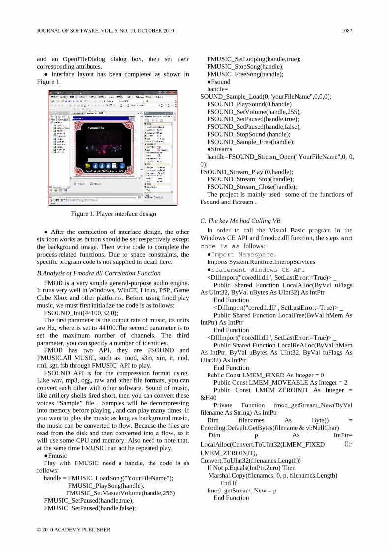
Figure 1. Player interface design

and an OpenFileDialog dialog box, then set their corresponding attributes. Interface layout has been completed as shown in

Figure 1.

After the completion of interface design, the other six icon works as button should be set respectively except the background image. Then write code to complete the process-related functions. Due to space constraints, the specific program code is not supplied in detail here.

B.Analysis of Fmodce.dll Correlation Function FMOD is a very simple general-purpose audio engine.

It runs very well in Windows, WinCE, Linux, PSP, Game Cube Xbox and other platforms. Before using fmod play music, we must first initialize the code is as follows:

FSOUND_Init(44100,32,0); The first parameter is the output rate of music, its units

are Hz, where is set to 44100.The second parameter is to set the maximum number of channels. The third parameter, you can specify a number of identities.

FMOD has two API, they are FSOUND and FMUSIC.All MUSIC, such as mod, s3m, xm, it, mid, rmi, sgt, fsb through FMUSIC API to play.

FSOUND API is for the compression format using. Like wav, mp3, ogg, raw and other file formats, you can convert each other with other software. Sound of music, like artillery shells fired short, then you can convert these voices “Sample” file. Samples will be decompressing into memory before playing , and can play many times. If you want to play the music as long as background music, the music can be converted to flow. Because the files are read from the disk and then converted into a flow, so it will use some CPU and memory. Also need to note that, at the same time FMUSIC can not be repeated play. Fmusic Play with FMUSIC need a handle, the code is as

follows: handle = FMUSIC_LoadSong("YourFileName");

FMUSIC_PlaySong(handle). FMUSIC_SetMasterVolume(handle,256)

FMUSIC_SetPaused(handle,true); FMUSIC_SetPaused(handle,false);

FMUSIC_SetLooping(handle,true); FMUSIC_StopSong(handle); FMUSIC_FreeSong(handle); Fsound handle=

SOUND_Sample_Load(0,"yourFileName",0,0,0); FSOUND_PlaySound(0,handle) FSOUND_SetVolume(handle,255); FSOUND_SetPaused(handle,true); FSOUND_SetPaused(handle,false); FSOUND_StopSound (handle); FSOUND_Sample_Free(handle); Streams handle=FSOUND_Stream_Open("YourFileName",0, 0,

0); FSOUND_Stream_Play (0,handle);

FSOUND_Stream_Stop(handle); FSOUND_Stream_Close(handle); The project is mainly used some of the functions of

Fsound and Fstream .

C. The key Method Calling VB In order to call the Visual Basic program in the

Windows CE API and fmodce.dll function, the steps and code is as follows: Import Namespace, Imports System.Runtime.InteropServices Statement Windows CE API <DllImport("coredll.dll", SetLastError:=True)> _ Public Shared Function LocalAlloc(ByVal uFlags

As UInt32, ByVal uBytes As UInt32) As IntPtr End Function <DllImport("coredll.dll", SetLastError:=True)> _ Public Shared Function LocalFree(ByVal hMem As

IntPtr) As IntPtr End Function <DllImport("coredll.dll", SetLastError:=True)> _ Public Shared Function LocalReAlloc(ByVal hMem

As IntPtr, ByVal uBytes As UInt32, ByVal fuFlags As UInt32) As IntPtr

End Function Public Const LMEM_FIXED As Integer = 0 Public Const LMEM_MOVEABLE As Integer = 2 Public Const LMEM_ZEROINIT As Integer =

&H40 Private Function fmod_getStream_New(ByVal

filename As String) As IntPtr Dim filenames As Byte() =

Encoding.Default.GetBytes(filename & vbNullChar) Dim p As IntPtr=

LocalAlloc(Convert.ToUInt32(LMEM_FIXED Or LMEM_ZEROINIT), Convert.ToUInt32(filenames.Length))

If Not p.Equals(IntPtr.Zero) Then Marshal.Copy(filenames, 0, p, filenames.Length) End If fmod_getStream_New = p End Function



Figure 2. the Interface layout in Eloidpxa27x

Friend WithEvents Panel1 As System.Windows.Forms.Panel

#End Region Statement Fmodce.dll function <DllImport("fmodce.dll",

EntryPoint:="FSOUND_Init", SetLastError:=True, CharSet:=CharSet.Unicode, CallingConvention:=CallingConvention.Winapi)> _ Public Shared Function fmod_Init(ByVal mixrate As Integer, ByVal maxsoftwarechannels As Integer, ByVal flags As Integer) As Boolean

End Function <DllImport("fmodce.dll",

EntryPoint:="FSOUND_Stream_GetLength", SetLastError:=True,CharSet:=CharSet.Unicode,CallingConvention:=CallingConvention.Winapi)> _ Public Shared Function fmod_GetLength(ByVal fstream As IntPtr) As Integer End Function

<DllImport("fmodce.dll", EntryPoint:="FSOUND_Stream_GetPosition", SetLastError:=True, CharSet:=CharSet.Unicode, CallingConvention:=CallingConvention.Winapi)> _ Public Shared Function fmod_GetPosition(ByVal fstream As IntPtr) As UInt32

End Function <DllImport("fmodce.dll", EntryPoint:="FSOUND_Stream_Open", SetLastError:=True, CharSet:=CharSet.Unicode, CallingConvention:=CallingConvention.Winapi)> _ Public Shared Function fmod_Open(ByVal data As IntPtr, ByVal mode As Integer, ByVal offset As Integer, ByVal length As Integer) As IntPtr

End Function <DllImport("fmodce.dll", EntryPoint:="FSOUND_Stream_Play", SetLastError:=True, CharSet:=CharSet.Unicode, CallingConvention:=CallingConvention.Winapi)> _ Public Shared Function fmod_Play(ByVal channel As Integer, ByVal fstream As IntPtr) As Integer


EntryPoint:="FSOUND_Stream_SetPosition", SetLastError:=True, CharSet:=CharSet.Unicode, CallingConvention:=CallingConvention.Winapi)> _

Public Shared Function fmod_SetPosition(ByVal fstream As IntPtr, ByVal position As UInt32) As Boolean


EntryPoint:="FSOUND_Stream_Stop", SetLastError:=True, CharSet:=CharSet.Unicode,

CallingConvention:=CallingConvention.Winapi)> _ Public Shared Function fmod_Stop(ByVal fstream

As IntPtr) As Boolean End Function <DllImport("fmodce.dll",

EntryPoint:="FSOUND_Close", SetLastError:=True, CharSet:=CharSet.Unicode, CallingConvention:=CallingConvention.Winapi)> _

Public Shared Sub fmod_Close() End Sub Private Function fmod_getStream(ByVal filename

As String) As IntPtr Dim filenames As Byte() =

Encoding.Default.GetBytes(filename & vbNullChar) Dim hfile As GCHandle =

GCHandle.Alloc(filenames, GCHandleType.Pinned) If Environment.Version.Major = 1 Then fmod_getStream = New

IntPtr(hfile.AddrOfPinnedObject().ToInt32 + 4) Else fmod_getStream = hfile.AddrOfPinnedObject() End If If hfile.IsAllocated Then hfile.Free() End If End Function #End Region Do a good job after the above two steps can use

Fmodce.dll function, combined with the control layout to achieve FmodMp3 player functions.

D.Change the target device platform The player program is based on the ARM architecture,

the program need no change when it is migrated to the real target device EEloidpxa27x embedded development board, the program can be downloaded to EEloidpxa270 development board if player device is selected. The interface when player in the development board run is shown in Figure 2. Next, transplant the project's program to Samsung smartphone I908E, before this, the program running environment should be simulated by Microsoft's Windows Mobile 6 emulator because of the reason that

Samsung's smartphone I908E is using a Windows Mobile 6.1 operating system. The following changes to the procedures applicable to smartphone available on the simulator program.

The most important first step is that, the project Properties has item "Change the target platform" only in the program written by managed Language (precisely, the intelligent devices platform with the same .NET Compact Framework version).As shown in Figure 3.



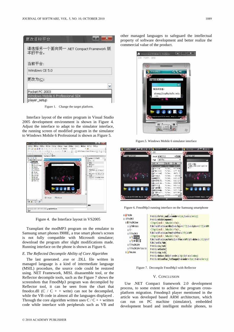
Figure 1. Change the target platform.

Interface layout of the entire program in Visual Studio

2005 development environment is shown in Figure 4. Adjust the interface to adapt to the simulator interface, the running screen of modified program in the simulator to Windows Mobile 6 Professional is shown as Figure 5.

Figure 4. the Interface layout in VS2005

Transplant the modMP3 program on the emulator to Samsung smart phones I908E, a true smart phone's screen is not fully compatible with Microsoft simulator; download the program after slight modifications made. Running interface on the phone is shown as Figure 6.

E. The Reflected Decompile Ability of Core Algorithm The last generated. .exe or .DLL file written in

managed language is a kind of intermediate language (MSIL) procedure, the source code could be restored using. NET Framework, MISL disassemble tool, or the Reflector decompile tools, such as the Figure 7 shows the screenshots that FmodMp3 program was decompiled by Reflector tool, it can be seen from the chart that fmodce.dll (C / C + + write) can not be decompiled, while the VB code in almost all the languages displayed . Through the core algorithm written uses C / C + + written code while interface with peripherals such as VB and

other managed languages to safeguard the intellectual property of software development and better realize the commercial value of the product.

Figure.5. Windows Mobile 6 simulator interface

Figure 6. FmodMp3 running interface on the Samsung smartphone

Figure 7. Decompile FmodMp3 with Reflector

V. CONCLUSION

Use .NET Compact framework 2.0 development process, to some extent to achieve the program cross-platform migration. Fmodmp3 player mentioned in the article was developed based ARM architecture, which can run on PC machine (simulator), embedded development board and intelligent mobile phones, to



achieve cross-platform migration. But some features can not be fully realized, this is caused by the reason that .NET framework is not supported in the .NET Compact framework exception mechanism and security mechanism. The design used only for the unique function of intelligent devices is also a relationship. But With the.NET Compact framework3.5, VS2008 and other technological advances, such as the program in the intelligent device to achieve true cross-platform will not be far away.

ACKNOWLEDGMENT

The authors wish to thank the Scientific and technological research project Foundation of Guangdong Province contract 2008B080701007 and Natural Science Foundation of Guangdong Province for contract 9151042001000017 under which the present work was possible.

REFERENCES

[1] XUE DaLong, CHEN ShiDi, WANG Yun. Windows CE embedded systems development from basic to practice. Beijing: Electronic Industry Press, 2008

[2] JIANG Bo.Windows Embedded CE6.0 Program designed to combat [M]. Beijing: Mechanical Industry Press, 2009

[3] (U.S.A) Powers·L, Snell·M （wrote） ;LIU YanBo，XIAO Na ， JIA Han （ translated ） Visual Studio2005 technology collection (M). Beijing: Posts & Telecom Press, 2008.1

[4] (France）Smacchia. P. (wrote); SHI Fan (translated). C# and .NET2.0 Practice: Platform, language and framework [M]. Beijing: Posts & Telecom Press, 2008.1

[5] CE6 OAL you have to know something[OL]. http://blog.sina.com.cn/s/blog-537bca0100corr.html.

[6] Microsoft. Advanced P/Invoke on .NET Compact Framework [J/OL].MSDN Library.

[7] Microsoft. NET framework decompiles technology [J/OL].MSDN Library.

Jing .Zhang was born in Dalian city,Liaoning province, November 24, 1977.Zhang graduated from Shenyang University of Technology in July of 2000 and received a bachelor of engineering degree. Then entered Guangdong University of Technology and Received a Master of Engineering degree in July of 2003.The major field of study is embedded system and Artificial Intelligence.

Her current job is TEACHING and works in .Guangdong University of Foreign Studies. Previous publications are: Circuit analysis and electronic technology(Beijing: Machinery Industry Press,2007),WINCE operating system transplantation based Intel PXA270(Beijing: Micro Computer Information,2008),Development and design of SQL Server Mobile database(Shanghai:Computer Application and Software,2008) .Now she is interested in embedded system and Artificial Intelligence.

Xinguang .Li was born in Nanxian city, Hunan province, July 6, 1965. Li graduated from South China University of Technology in July of 1998 and received a Dr. Degree. The major field of study is embedded system and Artificial Intelligence.

His current job is TEACHING and works in .Guangdong University of Foreign Studies. Now he is interested in embedded system and Artificial Intelligence.



A Metrics Method for Software Architecture Adaptability

Hong Yang

School of Information Science and Technology Dalian Maritime University, Dalian, China


Rong Chen and Ya-qing Liu School of Information Science and Technology

Dalian Maritime University, Dalian, China Email: second.author, [email protected]

Abstract—Based on GQM(Goal Question Metric) approach, this paper presents a new process-oriented metrics for software architecture adaptability. This method extends and improves the GQM method. It develops process-oriented processes for metrics modeling, introduces data and validation levels, adds structured description of metrics, and defines new indexes of metrics. Index Terms—Goal Question Metric, software architecture, adaptability, metrics, Interval Analytic Hierarchy Process, Data Envelopment Analysis

I. INTRODUCTION

Metrics is a process that assigns numbers or symbols to the attributes of entities in the real world based on clearly defined rules. Software quality measurement technique is a quantitative reflection, and its fundamental purpose is to assess the individual and the system or to predict the future development. Only through metrics, software engineering can enter the scientific stage.

Because software architecture development is the first phase in the design process, therefore, the measure of the quality of architecture will help us determine the quality of the final software. As an aspect of architecture quality characteristics, adaptability has a certain degree of specificity. The current research on the adaptability is still imperfect, lacks qualitative and quantitative metrics index and systemic evaluation method.

The current architecture analysis and evaluation methods are mostly based on the scene technology. In order to analyze the quality attributes of architecture more accurately, the majority of researchers believe that the use of metrics in the architecture stage to evaluate attribute is one of more precise technology. It includes metrics options for the quality attributes, the scale of metrics and a set of metrics methods. We can do this in two ways: first, adapting the existing measurement techniques, such as the dynamic complexity and dynamic coupling used in the design and code level validated effective object-oriented indexes. Object-oriented adaptability metrics for software maintainability prediction is very effective, because the required data

must be collected from the source code. But in the architecture phase, the prototype system has not been developed, and there is no source code. Therefore the second method is that definition and validation new measurement indexes in accordance with the characteristics of architecture, improving the metrics process. At present, some scholars are doing in this area. GQM (goal question metric) is a good technology used to define new metrics process. Based on GQM approach, integrating the research status, this paper presents a new process-oriented metrics for software architecture adaptability.

II. GQM

GQM (Goal Question Metric) is a widely used metrics modeling method. GQM is a goal-oriented (goal-oriented) method for software products and process metrics from Professor Victor Basisli of Maryland University. GQM refined goal to metrics by stepwise refinement approach, summarized and decomposed the objectives of the organization to metrics indexes, and refined these indexes to the value which can be measured. It is a goal-oriented metrics methods and a scientific and logical way of thinking for managers too.

The principle of the GQM approach is providing a model to help software managers to design a set of software metrics system for the management objectives, reduce and integrate the various objectives of software process and product model by systematic approach. GQM approach has strong flexibility and maneuverability. Implementation process is top-down analysis and bottom-up implementation process. First metrics target G (Goal) is putted forward, refining the goal to specific issue of Q (Question) of the process or product, and these questions can be answered in the way of measure M (Metric). So these vague and abstract goals are broken down into specific and measurable problems. Generally it is divided into three phases: the establishment of GQM metrics plan, the implementation of metrics and summarization of experiences. Each stage is divided into a number of activities. GQM measurement plan includes the early



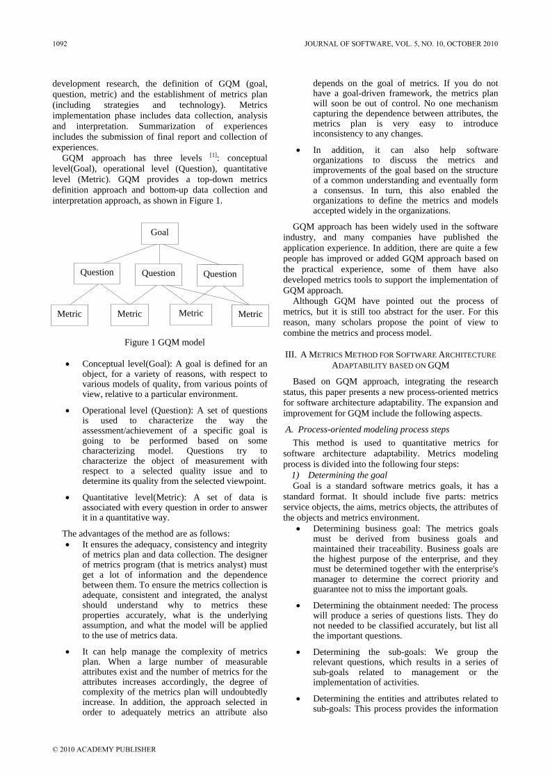
development research, the definition of GQM (goal, question, metric) and the establishment of metrics plan (including strategies and technology). Metrics implementation phase includes data collection, analysis and interpretation. Summarization of experiences includes the submission of final report and collection of experiences.

GQM approach has three levels [1]: conceptual level(Goal), operational level (Question), quantitative level (Metric). GQM provides a top-down metrics definition approach and bottom-up data collection and interpretation approach, as shown in Figure 1.

Figure 1 GQM model

Conceptual level(Goal): A goal is defined for an

object, for a variety of reasons, with respect to various models of quality, from various points of view, relative to a particular environment.

Operational level (Question): A set of questions is used to characterize the way the assessment/achievement of a specific goal is going to be performed based on some characterizing model. Questions try to characterize the object of measurement with respect to a selected quality issue and to determine its quality from the selected viewpoint.

Quantitative level(Metric): A set of data is associated with every question in order to answer it in a quantitative way.

The advantages of the method are as follows: It ensures the adequacy, consistency and integrity

of metrics plan and data collection. The designer of metrics program (that is metrics analyst) must get a lot of information and the dependence between them. To ensure the metrics collection is adequate, consistent and integrated, the analyst should understand why to metrics these properties accurately, what is the underlying assumption, and what the model will be applied to the use of metrics data.

It can help manage the complexity of metrics plan. When a large number of measurable attributes exist and the number of metrics for the attributes increases accordingly, the degree of complexity of the metrics plan will undoubtedly increase. In addition, the approach selected in order to adequately metrics an attribute also

depends on the goal of metrics. If you do not have a goal-driven framework, the metrics plan will soon be out of control. No one mechanism capturing the dependence between attributes, the metrics plan is very easy to introduce inconsistency to any changes.

In addition, it can also help software organizations to discuss the metrics and improvements of the goal based on the structure of a common understanding and eventually form a consensus. In turn, this also enabled the organizations to define the metrics and models accepted widely in the organizations.

GQM approach has been widely used in the software industry, and many companies have published the application experience. In addition, there are quite a few people has improved or added GQM approach based on the practical experience, some of them have also developed metrics tools to support the implementation of GQM approach.

Although GQM have pointed out the process of metrics, but it is still too abstract for the user. For this reason, many scholars propose the point of view to combine the metrics and process model.

III. A METRICS METHOD FOR SOFTWARE ARCHITECTURE ADAPTABILITY BASED ON GQM

Based on GQM approach, integrating the research status, this paper presents a new process-oriented metrics for software architecture adaptability. The expansion and improvement for GQM include the following aspects.

A. Process-oriented modeling process steps This method is used to quantitative metrics for

software architecture adaptability. Metrics modeling process is divided into the following four steps:

1) Determining the goal Goal is a standard software metrics goals, it has a

standard format. It should include five parts: metrics service objects, the aims, metrics objects, the attributes of the objects and metrics environment.

Determining business goal: The metrics goals must be derived from business goals and maintained their traceability. Business goals are the highest purpose of the enterprise, and they must be determined together with the enterprise's manager to determine the correct priority and guarantee not to miss the important goals.

Determining the obtainment needed: The process will produce a series of questions lists. They do not needed to be classified accurately, but list all the important questions.

Determining the sub-goals: We group the relevant questions, which results in a series of sub-goals related to management or the implementation of activities.

Determining the entities and attributes related to sub-goals: This process provides the information

Goal

Question Question Question

Metric Metric Metric Metric



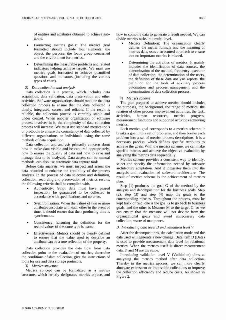
of entities and attributes obtained to achieve sub-goals.

Formatting metrics goals: The metrics goal formatted should include four elements: the object, the purpose, the focus group concerned and the environment for metrics.

Determining the measurable problems and related indicators helping achieve targets: We must use metrics goals formatted to achieve quantified questions and indicators (including the various types of chart).

2) Data collection and analysis Data collection is a process, which includes data

acquisition, data validation, data preservation and other activities. Software organizations should monitor the data collection process to ensure that the data collected is timely, integrated, correct and reliable. If the result is reliable, the collection process is certainly stable and under control. When another organization or software process involves in it, the complexity of data collection process will increase. We must use standard metrics tools or protocols to ensure the consistency of data collected by different organizations or individuals using the same methods of data acquisition.

Data collection and analysis primarily concern about how to make data visible and be captured appropriately, how to ensure the quality of data and how to save and manage data to be analyzed. Data access can be manual methods, can also use automatic data capture tools.

Before data analysis, we must inspect and assess the data recorded to enhance the credibility of the process analysis. In the process of data selection and definition, collection, recording and preservation of metrics results, the following criteria shall be complied with.

Authenticity: Strict data must have passed inspection, be guaranteed to be collected in accordance with specifications and no error.

Synchronization: When the values of two or more attributes associate with each other in the event of time, it should ensure that their producing time is synchronous.

Consistency: Ensuring the definition for the record values of the same type is same.

Effectiveness: Metrics should be clearly defined to ensure that the value used to describe an attribute can be a true reflection of the property.

Data collection provides the data flow from data collection point to the evaluation of metrics, determine the conditions of data collection, give the instructions of tools for use and data storage protocols.

3) Metrics structure Metrics concept can be formalized as a metrics

structure, which strictly designates metrics objects and

how to combine data to generate a result needed. We can divide metrics tasks into multi-level.

Metrics Definition: The organization clearly defines the metric formula and the meaning of metrics data, uses a structured approach to ensure that no important metrics is missed.

Determining the activities of metrics: It mainly includes the identification of data sources, the determination of the method, frequency, executor of data collection, the determination of the users, the definition of these data analysis reports, the definition for the tools of auxiliary process automation and process management and the determination of data collection process.

4) Metrics scheme The plan prepared to achieve metrics should include:

the purposes, the background, the range of metrics, the relation of other process improvement activities, the task, activities, human resources, metrics progress, measurement functions and supported activities achieving metrics.

Each metrics goal corresponds to a metrics scheme. It breaks a goal into a set of problems, and then breaks each problem into a set of metrics process descriptions. It is a necessary process, which defines specific attributes to achieve the goals. With the metrics scheme, we can make specific metrics and achieve the objective evaluation by analyzing the metrics data sequentially.

Metrics scheme provides a consistent way to identify, select and specify the information needed by software architecture adaptation. And it integrates them into the analysis and evaluation of software architecture. The result of metrics scheme is the achievement of metrics plan.

Step (1) produces the goal G of the method by the analysis and decomposition for the business goals. Step (2), step (3) and step (4) map the goals to the corresponding metrics. Throughout the process, must be kept track of two: one is the goal G to go back to business goals, and the other is Measure M to the target G, so we can ensure that the measure will not deviate from the organizational goals and avoid unnecessary data collection, waste of manpower.

B. Introducing data level D and validation level V After the decompositions, the calculation mode and the

data used will generate a new change. Data item D (Data) is used to provide measurement data level for relational metrics. When the metrics itself is direct measurement data, D and M are the same.

Introducing validation level V (Validation) aims at analyzing the metrics method after data collection. Thereby in the metrics process, we can more clearly abnegate excrescent or impossible collections to improve the collection efficiency and reduce costs. As shown in Figure 2.



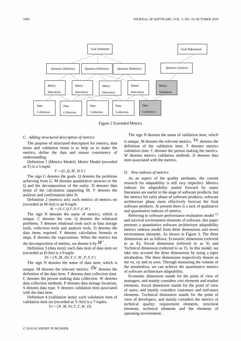
C. Adding structured description of metrics The purpose of structured description for metrics, data

items and validation items is to help us to make the metrics, define the data and ensure consistency of understanding.

Definition 1 (Metrics Model): Metric Model (recorded as T) is a 5-tuple.

( , , , , )T G Q M D V The sign G denotes the goals. Q denotes the problems

achieving from G. M denotes quantitative answers to the Q and the decomposition of the entity. D denotes data items of the calculation supporting M. V denotes the analysis and confirmation after D.

Definition 2 (metrics set): each metrics of metrics set (recorded as M-Set) is an 8-tuple.

( , , , , , , , ')iM N C Q T D F E M The sign N denotes the name of metrics, which is

unique. C denotes the cost. Q denotes the relational problems. T denotes relational tools such as data storage tools, collection tools and analysis tools. D denotes the data items required. F denotes calculation formula or steps. E denotes the expectations. When the metrics has the decomposition of entities, we denote it by 'M .

Definition 3 (data item): each data item of data item set (recorded as D-Set) is a 9-tuple.

( , , , , , , , , )Di N M De T C W P S V The sign N denotes the name of data item, which is

unique. M denotes the relevant metrics. De denotes the definition of the data item. T denotes data collection time. C denotes the person making data collection. W denotes data collection methods. P denotes data storage locations. S denotes data type. V denotes validation item associated with the data item.

Definition 4 (validation item): each validation item of validation item set (recorded as V-Set) is a 7-tuples.

V ( , , , , , , )i N M Ve T C W D

The sign N denotes the name of validation item, which is unique. M denotes the relevant metrics. Ve denotes the definition of the validation item. T denotes metrics validation time. C denotes the person making the metrics. W denotes metrics validation methods. D denotes data item associated with the metrics.

D. New indexes of metrics As an aspect of the quality attributes, the current

research for adaptability is still very imperfect. Metrics indexes for adaptability putted forward by many literatures are useful in the stage of software products, but the metrics for early phase of software products, software architecture phase more effectively forecast the final software products. At present there is a lack of qualitative and quantitative indexes of metrics.

Referring to software performance evaluation model [2] and survival environment elements of software, this paper presents a quantitative software architecture adaptability metrics indexes model from three dimensions and seven environment elements. As shown in Figure 3. The three dimensions are as follows: Economic dimension (referred to as E), Social dimension (referred to as S) and Technical dimension (referred to as T). In this model, we take into account the three dimensions by using a taper tetrahedron. The three dimensions respectively denote as the ox, oy and oz axes. Through measuring the volume of the tetrahedron, we can achieve the quantitative metrics of software architecture adaptability.

Economic dimension stands for the point of view of managers, and mainly considers cost elements and market elements. Social dimension stands for the point of view of users, and mainly considers customers and end-users elements. Technical dimension stands for the point of view of developers, and mainly considers the metrics of technical quality: requirement elements, structural elements, technical elements and the elements of operating environment.

Goal Statement

Question Definition Question Definition Question Definition

Metric

Derivation

Metric

Derivation

Metric

Derivation

Metric

Derivation

Data

Collection

Data

Collection

Data

Collection

Data

Collection

Data

Collection

Metric

Validation

Question Analysis

Goal Refinement

Figure 2 Extended Metrics



Figure 3 three-dimension metrics indexes model for software architecture adaptability

E. Decision-making method based on IAHP and DEA AHP put forward by a famous expert of operational

research in America is a practical and multi-properties decision making method. This method combines qualitative and quantitative analysis to deal with various decision-making elements. It is systemic, flexible and terse and applied in the social and economic fields quickly and widely. The traditional AHP uses an exact number to show the judgment that the expert make when they compare the two projects. But it is difficult for a decision-making expert to do this in the practical situation. The problem we meet is more complicated and sensitive and the known information is not all-sided and assured enough. Therefore, there is uncertainty and subjectivity when the expert makes a comparison between the two projects. In order to solve these problems, IAHP comes into being. It uses interval number instead of point value to form judgment matrix and then get the interval weight vector. The original data and result are also expressed by interval numbers so that the flexible decision realizes. In the interval AHP, decision-making expert can ascertain the importance of various elements but there is disaccord in judgment matrix. While DEA is a new method of evaluating efficiency based on the idea of relative efficiency. It is one of the effective ways of dealing with multi-goals decision-making problems. CCR model of DEA adopts variation weights to evaluate the decision-making item on the base of input and output data. It just focuses on the status value of the considered elements corresponding to the decision-made objects. Therefore, the combining of the both can give a reasonable decision-making method to solve the above problems.

The traditional combining of AHP and DEA are most often adopted. Either point weights [14-17] or interval weights [18] are regarded as constraints. Based on this, this paper improves the method given by literature [14-17] , uses interval number to express the original data and result, makes the interval weight vector constraints, emphasizes on the differences between AHP and DEA and their own advantages. It provides a new thought for multi-goals

decision-making problems and uses an example of practical application to show its effectiveness.

1) Algorithm Suppose the number of the objects of the same type is

n. The objects are arranged according to the status value that each object has in the m aspects. The bigger the status value of these elements is, the better it is.

The first step: use IAHP [19-20] to get the right weights of these S kinds of elements.

For the influence of various uncertain elements, it is difficult for the decision-making experts to use an exact number to show the judgment they make after the comparison between the two projects. The experts can only give a range in the form of interval. That is aij ＝

ij ija ,a . It denotes the judgment the experts make after comparing the importance of the project I and J. Here,

ij ija a、separately refers to the upper limit and lower limit.

Thereupon, the comparison judgment matrix of these n elements goes like this:

12 12 1 1

2 2

1 , ,

1 ,A1

1

n n

n n

a a a a

a a

＝

(1)

In the formula

1ij

ij

aa

>0 ，

1ii iia a ，

1 99 ij ija a

，i,j=1,2,…,n，A is called the interval judgment matrix. The interval judgment matrix A is a

reciprocal. If to all i,j=1,2,…,n， ij ija a, A contracts to

the traditional point judgment matrix. Suppose the interval weight is

Wi=[ ii ， ](i=1,2,…,n). According to the operation

principle of interval number, there is

,i i i

j jj

WW

.

Thus it can be seen when getting the interval weight vector of the judgment matrix, the distance between

ijaand

i

j

, ijaand

i

j

should be as short as possible in order to make the uncertainty degree of the vector as small as possible. For the mutual-opposite of the judgment matrix, only upper triangular matrix can be



taken into account when considering the judgment matrix. Using external approximation computation, that is, if to all i and j, wij includes the judgment interval aij, then

i iij ij

jj

a a

，

, 1≤i<j≤n (2) In order to make the interval weight vector satisfy the

standard as the traditional point weight vector, the theorem of the standard interval vector proposed by the reference can be adopted:

1 1

1, 1n n

j i j ii ii j i j

, j＝1,2,…,n (3)

The interval weight computation is the core of IAHP.

The present computation methods are mainly iterative method 、 stochastic simulation method 、 interval eigenvalue method、mutual-complement matrix method and linear programming method etc. This article adapts LP to get the interval weight by combining formula (2) and (3). LP model is just the following:

min 1

n

i ii

s.t.

i iij ij

jj

a a

，

，i=1,2,…,n-1; j=i+1,i+2,…,n (4)

1 1

1, 1n n

j i j ii ii j i j

, j＝1,2,…,n

i i i=1,2,…,n The second step: the second consideration on the

weight of mi(i=1,2,…,s) items are transferred to the one on the sequence of status value of these decision-made objects by using CCR model of DEA[18].

DMU is used to refer to the objects of the same type. The bigger the status value of these items is, the better it is. status value is regarded as the output index. Suppose there is an input index in which all the objects meet one requirement, and all the input data is 1.

Suppose the efficiency evaluation of DMUjo is made. The weight of input index V and the weight of output

index ir 1 ku u ,u2, ,u＝ are variables. The

efficiency index of jo DMU is the target. The efficiency

of all DMU j

s

rjr

vx

yu1r

jh＝≤1 (j=1,2,…,n; r=1,2,…,ki) is

the constraint. Then the most optimized model is formed. After the change of C2 (Charnes-Cooper), the following linear programming model is set up:

io

=max uyo s.t. vxo=1 (5)

-vX+uY≤0 v≥0, u≥0

In this formula,

)1,,1,1(,,,xX 21 nxx＝ represents input index, xj is the input result that can be obtained when the j DMU corresponds to this input index.

snss

n

n

yyy

yyyyy

21

22221

11211y

Y＝

represents output index, yrj is the output result when the J DMU corresponds to R output index; v and u represents input weight and output weight respectively.

After canonicity transforms the output data through yrj/yor, we can get

11 1

21 2

1

ˆ ˆy 1ˆ ˆ1

Y

ˆ ˆ1

n

n

s sn

yy y

y y

＝

Then:

ij 1 2 rˆ ˆ ˆ ˆu u u ＝

i=1,2,…,s; j=1,2,…,n；r=1,2,…,ki (6)

ij

can be regarded as the sequence weights of the jth object in n items according to the status value of this kind of elements. The interval weight of this class can also be considered.

The third step: The weights of the decision-made items in all the considered items can be confirmed by combining the results gained by the first and second step, that is, by adding the interval weights constraints of the interval AHP in DEA evaluation model. Therefore, the decision-making experts can get the final sequence of all the items.

Suppose the interval weights of the output index

gained by interval AHP is [ r r ， ], then



1

ˆ

î

rr rk

rr

uw wu

r=1,2,…,ki (7)

Combining formula (5) and (7) can get

io

=max 1

îk

rr

u

s.t. ûY 1 (8)

1

ˆ

î

rr rk

rr

uw wu

r=1,2,…,ki

u 0

The weights of the decision-made projects in all considered objects can be gained in accordance with status value of all the elements by formula (8).

2) Computation example Suppose one decision-making problem. There is one

input index, four output index and five decision-made objects. The judgment matrix of the output index given by decision-making experts after comparing each two is like the following:

1 1 1 11 , 3,6 ,6 4 4 2

1 6,8 2,4A

1 11 ,8 6

1

＝

The specific data of these five objects is like this:

x1 y1 y2 y3 y4

The whole process is like this: （1）The linear programming model can be set up by

matrix A according to the formula (4) and the result can be obtained by software LINDO. The optimal value z=0.3.

Thus , the interval weights vector of A is [0.075,0.15]，[0.6,0.6]，[0.025,0.1]，[0.15,0.3].

（2）The original linear programming model can be

set up by the specific data of the objects according to the formula (5).

The evaluation index of the most superior efficiency is

1o 2 3 4 5o o o o ＝1.00，＝0.85，＝1.00，＝1.00，＝1.00

. （3）The object A is taken as an example. The data is

gained like the following by making the output data canonicity transforms through yrj/yor.

A B C D Ey1 1 2 2 3 3 y2 1 0.375 0.75 0.375 0.875y3 1 4 6 5 4 y4 1 1.333 0.333 1.667 0.667

According to formula (8), the linear programming

model can be set up. The evaluation index of the most

superior efficiency can be gained. That is 1o ＝0.930 . The weights of the index output are respectively [0.075, 0.6, 0.025, 0.3].

In the same way, the other evaluation indexes are

2 3 4 5ˆ ˆ ˆ ˆ

o o o o ＝0.552，＝0.736，＝0.568，＝1.000 . Therefore, the final sequence of these five objects is E、A、C、D、B.

IV. CONCLUSION

Based on GQM approach, integrating the research status, this paper presents a new process-oriented metrics for software architecture adaptability. This method extends and improves the GQM method. It develops process-oriented processes for metrics modeling, introduces data and validation levels, adds structured description of metrics, and defines new indexes of metrics. The method resolves the metrics for software architecture adaptability to some extent. However, it is still insufficient, needs further in-depth study.

ACKNOWLEDGMENT

This work was supported by the National Natural Science Foundation of China under Grant No.60775028 and the Key Project of Science and Technology Board of Dalian of China under Grant No. 2007A14GX042.

A 1 1 8 1 3 B 1 2 3 4 4 C 1 2 6 6 1 D 1 3 3 5 5 E 1 3 7 4 2

y1 y2 y3 y4

y1

y2

y3

y4



REFERENCES

[1] Basili V R, Caldiera1 G, Rombach HD. The goal question metric approach.1994

[2] Buglione L, Abran A. Geometrical and statistical foundations of a three-dimensional model of software performance. Advances in engineering software,1999(30):913-919

[3] Olsson T, Runeson P. V-GQM: A Feed-Back approach to validation of a GQM study. 7th international software metrics symposium IEEE, 2001,4(4-6):236-245.

[4] Basili, Heidrich J. GQM + strategies-aligning business strategies with software measurement. The first international symposium on empirical software engineering and measurement, 2007.

[5] Montini D A. Using GQM hypothesis restriction to infer Bayesian network testing. The sixth international conference on information technology, 2009.

[6] Knauss E, EI Boustani C. Assessing the quality of software requirements specifications. The 16th IEEE international requirements engineering, 2008.

[7] Subramanian N, Chung L. Metrics for software adaptability.2000

[8] Aversano L. A framework for measuring business processes based on GQM. The 37th annual hawai international conference on system sciences, 2004.

[9] Birk, A., van Solingen, R., Jarvinen, J. Business Impact, Benefit and Cost of Applying GQM in Industry: An In-Depth, Long-Term Investigation at Schlumberger RPS. 5th International Software Metrics Symposium IEEE, 1998,11(20-21): 93-96.

[10] Niessink F, van Vliet H. Measurements Should Generate Value, Rather Than Data. 6th International Software Metrics Symposium IEEE, 1999,11(4-6):31-38.

[11] Offen R J, Jeffery R. Establishing Software Measurement Programs. Software IEEE, 1997,14(2): 45-53.

[12] van Solingen R, Berghout E. Integrating Goal-Oriented Measurement in Industrial Software Engineering: Industrial Experiences with and Additions to the Goal/Question/Metric Method (GQM). 7th International Software Metrics Symposium IEEE, 2001,4(4-6):246-258.

[13] Bianchi A J. Management Indicators Model to Evaluate Performance of IT Organizations. Management of engineering and technology, 2001,2(29):217-229.

[14] Wang Ying-ming, Liu Jun, Elhag Taha M S, an integrated AHP-DEA methodology for bridge risk assessment, Computers and Industrial Engineering, 2008,54(3):513-525

[15] Azadeh A, Ghaderi S F, Lzadbakhsh H, Integration of DEA and AHP with computer simulation for railway system improvement and optimization, Applied Mathematics and Computation, 2008,195(2):775-785

[16] Lin Ji-keng, Jiang Yue-mei, Yue Shun-min, Assessment of effective schemes for power system blackstart based on DEA/AHP, Dianli Xitong Zidonghua/Automation of Electric Power Systems, 2007,31(15):65-69

[17] Guo Jing-yuan, Liu Jia, Qiu li, Research on supply chain performance evaluation based on DEA/AHP model, Proceedings of 2006 IEEE Asia-Pacific Conference on Services Computing, APSCC, p 609-612,2006

[18] Entani T, Ichihashi H, Tanaka H, Evaluation method based on interval AHP and DEA, physica-Verlag CEJOR, 25-34 no.12, pp.25-34, 2004

[19] Entani T, Tanaka H, Interval estimations of global weights in AHP by upper approximation, Fuzzy Sets and Systems, 2007,158(17):1913-1921

[20] Li Cheng-ren, Comprehensive post-evaluation of rural electric network reformation based on fuzzy interval number AHP, Proceedings of International Conference on Risk Management and Engineering Management, p 171-177, 2008



ARM Static Library Identification Framework

Qing Yin, Fei Huang, Liehui Jiang National Digital Switching System Engineering & Technology Research Center

1001-718#, Zhengzhou, Henan Province 450002, China [email protected]

Abstract—A static library identification framework is proposed through studying library as “dcc”, which dynamically extracts binary characteristic file on applications under ARM processor. This framework obtains function modules according to ARM assemble characteristics, on the basis of which dynamic signature is generated due to pattern files through analyzing coding characteristics of assemble addressing mode and that of corresponding binary codes, then signatures of candidate functions are matched with signatures of library functions using hash algorithm to identify library functions. This method can recognize library functions efficiently and solve conflict between massive library files and matching efficiency effectively. Index Terms—library function; ARM; pattern matching; characteristic signature

I. INTRODUCTION

Decompilation is one technique that can translate object codes into corresponding high-level language expression. Then, the static linked library functions in legacy software are difficult to decompile because of whose own code characteristics, and static library functions are code modules which are linked statically and depend on compilers, so it is beneficial for decreasing the work of decompilation and increasing validity and readability of identification to recognize static library function modules, which is good to understand program intention and analyzing program’s key parts.

Embedded devices are applied abroad in every fields, and its processor types are over one thousand so far. Now microprocessors applied ARM technique mainly take up over 70 percent of RISC microprocessor’ share, whose market is broad. However, the related literatures at home and abroad of library identification concentrated on ARM processor are few, while the requirement of reuse, development and key functions’ extraction of legacy software are increasingly urgent.

Static library functions are function modules that are embedded into program in function body form, while dynamic library functions are function modules that are applied dynamically. The form of library function existing in executables is close to processor architecture [1]. Static library functions are compiled by compiler of special version, so library files of different version’ compilers vary in formation and content.

Existing static library functions identification method on ARM is relatively few, most are for x86 processor, which firstly extracts characteristic library, then compares extracted function modules with characteristic library to fulfill identification. According to characteristic extracting level, there are mainly two aspects: (1) Library functions pattern extraction based on

intermediate code level; 8086C decompiler brings out a method that includes library functions’ main characteristics and secondary characteristics, then to generate pattern table. According to different characteristics, eight matching methods are proposed. This method is very strict in theory and complex in application. On the basis of disassembling library functions, Mr. Li Xiang Yang extracts library pattern on intermediate code level, which is matched with candidate function modules [2]. The arithmetic is simply fast, but its weak point is ignoring the characteristic of operand and addressing type and clashes during match process.

(2) Library functions pattern extraction based on object code level; IDA and DCC use FLIRT technique, which generates pattern files using first n bytes of object programs, on the basis of which binary pattern library [3] is generated. The signature is obtained by hashing pattern files in library, which will be matched in matching process. This method results effective and efficient, and can recognize static library functions in object codes well.

On analyzing static library function identification arithmetic of x86 processor, combined with coding characteristic of ARM architecture in executables, a library function identification arithmetic on ARM whose characteristic length can be defined is proposed. ARM static library function identification apply extracting binary coding of library to fulfill the uniqueness and integrality of characteristic obtaining, using hash arithmetic to fulfill the automation and efficiency of matching process, using characteristic length that can be defined to fulfill the control of matching precision.

II. STATIC LIBRARY RECOGNITION MODEL

Static library functions’ popular process is as Figure. 1 [4]:

Library function recognition model generally contains four modules:



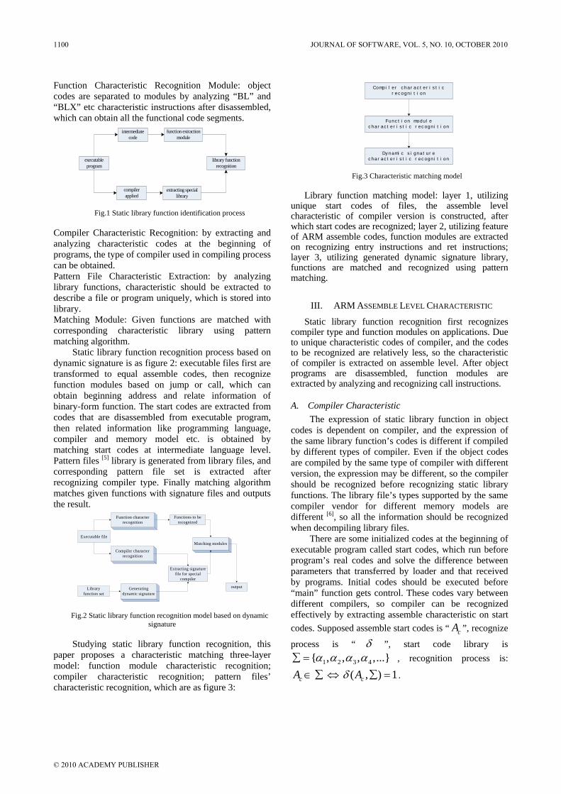
Function Characteristic Recognition Module: object codes are separated to modules by analyzing “BL” and “BLX” etc characteristic instructions after disassembled, which can obtain all the functional code segments.

intermediate code

extracting special library

library function recognition

compiler applied

executable program

function extraction module

Fig.1 Static library function identification process

Compiler Characteristic Recognition: by extracting and analyzing characteristic codes at the beginning of programs, the type of compiler used in compiling process can be obtained. Pattern File Characteristic Extraction: by analyzing library functions, characteristic should be extracted to describe a file or program uniquely, which is stored into library. Matching Module: Given functions are matched with corresponding characteristic library using pattern matching algorithm.

Static library function recognition process based on dynamic signature is as figure 2: executable files first are transformed to equal assemble codes, then recognize function modules based on jump or call, which can obtain beginning address and relate information of binary-form function. The start codes are extracted from codes that are disassembled from executable program, then related information like programming language, compiler and memory model etc. is obtained by matching start codes at intermediate language level. Pattern files [5] library is generated from library files, and corresponding pattern file set is extracted after recognizing compiler type. Finally matching algorithm matches given functions with signature files and outputs the result.

Executable file

Function character recognition

Compiler character recognition

Library function set

Generating dynamic signature

Extracting signature file for special

compiler

Functions to be recognized

Matching modules

output

Fig.2 Static library function recognition model based on dynamic

signature

Studying static library function recognition, this paper proposes a characteristic matching three-layer model: function module characteristic recognition; compiler characteristic recognition; pattern files’ characteristic recognition, which are as figure 3:

Compi l e r c ha r a c t e r i s t i c r e c ogni t i on

Dy nami c s i gna t ur e c ha r a c t e r i s t i c r e c ogn i t i on

F unc t i on modul e c ha r a c t e r i s t i c r e c ogni t i on

Fig.3 Characteristic matching model

Library function matching model: layer 1, utilizing unique start codes of files, the assemble level characteristic of compiler version is constructed, after which start codes are recognized; layer 2, utilizing feature of ARM assemble codes, function modules are extracted on recognizing entry instructions and ret instructions; layer 3, utilizing generated dynamic signature library, functions are matched and recognized using pattern matching.

III. ARM ASSEMBLE LEVEL CHARACTERISTIC

Static library function recognition first recognizes compiler type and function modules on applications. Due to unique characteristic codes of compiler, and the codes to be recognized are relatively less, so the characteristic of compiler is extracted on assemble level. After object programs are disassembled, function modules are extracted by analyzing and recognizing call instructions.

A. Compiler Characteristic The expression of static library function in object

codes is dependent on compiler, and the expression of the same library function’s codes is different if compiled by different types of compiler. Even if the object codes are compiled by the same type of compiler with different version, the expression may be different, so the compiler should be recognized before recognizing static library functions. The library file’s types supported by the same compiler vendor for different memory models are different [6], so all the information should be recognized when decompiling library files.

There are some initialized codes at the beginning of executable program called start codes, which run before program’s real codes and solve the difference between parameters that transferred by loader and that received by programs. Initial codes should be executed before “main” function gets control. These codes vary between different compilers, so compiler can be recognized effectively by extracting assemble characteristic on start codes. Supposed assemble start codes is “ cA ”, recognize

process is “ δ ”, start code library is

1 2 3 4 , , , ,...α α α α∑ = , recognition process is:

cA ∈ ∑ ⇔ ( , ) 1cAδ ∑ = .



Fig.4 start codes of executable program

This paper extracts assemble level start code as signature, which is based on disassembling of executable program by IDA. The assemble codes between “_start” [7]

and “main” are module of recognizing compiler. Compiler characteristic library is constructed by extracting characteristic files from start codes of executable files, which will be matched when recognizing compiler’s type.

B. Function Module Characteristic Static library function recognition is matching with

embedded modules in executable programs. Due to compile optimization and relocation [8], library function may varies after compiled. So matching on object codes bit by bit is inaccurate, and object codes’ size may be relatively big. Rough matching may wastes lots of time and can’t fulfill good impact. So object codes should be disassembled and separated into function modules before matching, which gets all the function modules in executable programs and simplifies matching process.

The intermediate language codes for ARM don’t own “call” etc. instructions which call subroutines, and there are not “ret n” etc instructions to indicate end address of function. Function module recognition for ARM is fulfilled on assemble level, whose assemble codes’ features are as follows:

• Assemble codes for ARM are equal to object codes, which doesn’t have definite entry point like PE files when disassembling.

• The call to function modules in ARM assemble instructions is fulfilled by jump in program flow. The jump in flow is fulfilled by two kinds of instructions: special “jump” instruction; writing address value to “PC”.

• Subroutine’s call mainly applies “BL, BLX”, which stores the value of “PC” into an special register (R14) before jumping and recovers the value of “PC” before returning.

Function recognition algorithm is as follows: Function: recognizing address section of function modules Input: intermediate language codes for ARM Output: function module’s address section (b, e) Algorithm:

Fig.5 Function recognition algorithm

IV. DYNAMIC SIGNATURE

Signature file is a special format file that is generated when recognizing static library functions, which can be matched with functions recognized from executable files. On the basis of deeply analyzing library functions, every library function body is different to each other, and most of them are different on bytes of the beginning. So this paper extracts first n bytes of library as the characteristic codes of pattern files due to this feature.

A. Library Files Structure Characteristic ARM library files’ format under Linux mainly

contains share library(.so file) and static library(.a file). Static library files are library file that exist in “.a” format, which pack several object files(.o file) into a library file, the structure of which mainly contain the following parts:

File characteristic word (magic number): it is a string used for marking file structure, the length is 8, the value is “!<arch>\n”.

Section: “.a” file contains four type’s sections; first section, second section, longname section and obj section. The second section and longname section are optional, which may not appear in a file. Every section contains two parts: header and data parts.

The format of header is the same to each other, whose content are as follows: struct

char name[16]; // name char time[12]; // time char userid[6]; // user id char groupid[6]; //group id char mode[8]; // mode char size[10]; // length char endofheader[2]; // 结束符

sectionheader; First section is the first section of a file, the structure

of whose data part is as follows: struct

unsigned long symbolnum; // symbol number unsigned long symboloffset[n]; // object section offset

Cbegin = _start; Begin：

Code_scan = next line codes； If(Code_scan = null)

Return ; Scan（code section）；

If (there is not jump instruction incodes) Goto Begin;

Else Scan（later codes）

If（find “PC” value is set） Output（address sections）；

Goto Begin;



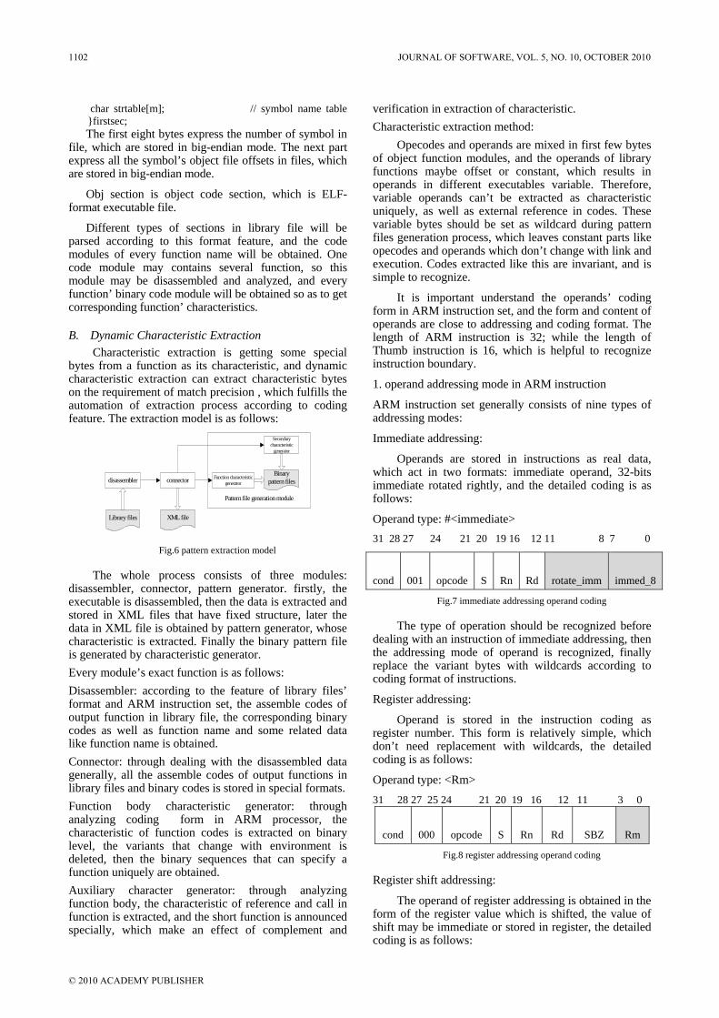
char strtable[m]; // symbol name table firstsec;

The first eight bytes express the number of symbol in file, which are stored in big-endian mode. The next part express all the symbol’s object file offsets in files, which are stored in big-endian mode.

Obj section is object code section, which is ELF-format executable file.

Different types of sections in library file will be parsed according to this format feature, and the code modules of every function name will be obtained. One code module may contains several function, so this module may be disassembled and analyzed, and every function’ binary code module will be obtained so as to get corresponding function’ characteristics.

B. Dynamic Characteristic Extraction Characteristic extraction is getting some special

bytes from a function as its characteristic, and dynamic characteristic extraction can extract characteristic bytes on the requirement of match precision , which fulfills the automation of extraction process according to coding feature. The extraction model is as follows:

Pattern file generation module

Library files

disassembler connector

XML file

Function characteristic generator

Binary pattern files

Secondary characteristic

generator

Fig.6 pattern extraction model

The whole process consists of three modules: disassembler, connector, pattern generator. firstly, the executable is disassembled, then the data is extracted and stored in XML files that have fixed structure, later the data in XML file is obtained by pattern generator, whose characteristic is extracted. Finally the binary pattern file is generated by characteristic generator. Every module’s exact function is as follows: Disassembler: according to the feature of library files’ format and ARM instruction set, the assemble codes of output function in library file, the corresponding binary codes as well as function name and some related data like function name is obtained. Connector: through dealing with the disassembled data generally, all the assemble codes of output functions in library files and binary codes is stored in special formats. Function body characteristic generator: through analyzing coding form in ARM processor, the characteristic of function codes is extracted on binary level, the variants that change with environment is deleted, then the binary sequences that can specify a function uniquely are obtained. Auxiliary character generator: through analyzing function body, the characteristic of reference and call in function is extracted, and the short function is announced specially, which make an effect of complement and

verification in extraction of characteristic. Characteristic extraction method:

Opecodes and operands are mixed in first few bytes of object function modules, and the operands of library functions maybe offset or constant, which results in operands in different executables variable. Therefore, variable operands can’t be extracted as characteristic uniquely, as well as external reference in codes. These variable bytes should be set as wildcard during pattern files generation process, which leaves constant parts like opecodes and operands which don’t change with link and execution. Codes extracted like this are invariant, and is simple to recognize.

It is important understand the operands’ coding form in ARM instruction set, and the form and content of operands are close to addressing and coding format. The length of ARM instruction is 32; while the length of Thumb instruction is 16, which is helpful to recognize instruction boundary.

1. operand addressing mode in ARM instruction

ARM instruction set generally consists of nine types of addressing modes:

Immediate addressing:

Operands are stored in instructions as real data, which act in two formats: immediate operand, 32-bits immediate rotated rightly, and the detailed coding is as follows:

Operand type: #<immediate> 31 28 27 24 21 20 19 16 12 11 8 7 0

cond 001 opcode S Rn Rd rotate_imm immed_8

Fig.7 immediate addressing operand coding

The type of operation should be recognized before dealing with an instruction of immediate addressing, then the addressing mode of operand is recognized, finally replace the variant bytes with wildcards according to coding format of instructions.

Register addressing:

Operand is stored in the instruction coding as register number. This form is relatively simple, which don’t need replacement with wildcards, the detailed coding is as follows:

Operand type: <Rm> 31 28 27 25 24 21 20 19 16 12 11 3 0

cond 000 opcode S Rn Rd SBZ Rm

Fig.8 register addressing operand coding

Register shift addressing:

The operand of register addressing is obtained in the form of the register value which is shifted, the value of shift may be immediate or stored in register, the detailed coding is as follows:



Operand type：<Rm>, <shift> <Rs>

28 24 21 20 19 16 12 11 8 7 6 5 4 3 0

cond opcode S Rn Rd Rs 0 Shift 1 Rm

Fig.9 register shift addressing operand coding by register

Operand type：<Rm>, <shift> #<shift_imm> 28 24 21 20 19 16 12 11 8 6 5 4 3 0

cond opcode Rn Rd Shift_imm Shift 0 Rm

Fig.10 register shift addressing operand coding by immediate

Register indirect addressing:

Register indirect instruction is usually applied in transmission instructions, whose register is stored as the address pointer of operand, which reflects in ARM coding the same as in register addressing, the coding is as follows:

Operand type：[<Rm>]

31 28 27 20 19 1615 12 11 0

cond Rn Rd addr_mode

Fig.11 register indirect addressing operand coding

Base plus offset addressing:

Base plus offset addressing is also called indexed addressing, offset value being 4KB, which is divided into three types: pre-indexed, auto-indexed, and post-indexed. The type of indexed addressing is decided by “P” bit and “W” bit. Among which operands have three types, register plus offset, register plus register, and register plus register shifted.

Operand type：[<Rn>, #+/-<offset_12>]

31 28 23 22 21 20 19 16 15 12 11 0

cond U B 1 L Rn Rd offset_12

Fig.12 immediate indexed operand coding

Operand type：[<Rn>, +/-<Rm>]

31 28 21 20 19 16 15 12 11 4 3 0

cond U B 1 L Rn Rd SBZ Rm

Fig.13 register indexed operand coding

Operand type：[<Rn>, +/-<Rm>, <shift> #<shift_imm>]

31 28 20 19 16 15 12 11 7 6 5 3 0

cond L Rn Rd shift_imm shift 0 Rm

Fig.14 shifted register indexed operand coding

Multi-register addressing:

The instruction that apply multi-register addressing can achieve the transformation of several registers, which may reach 16 at most.

Operand type：<registers>

31 28 24 23 22 21 20 19 16 15 0

cond P U 0 W 1 Rn Register——list

Fig.15 multi-register list operand coding

Stack addressing:

Stack addressing operate on data by visiting stack, which contains two types: the first is up increasing, the second is down increasing.

Operand type：<registers>

15 9 8 7 0

cond R Register——list

Fig.16 stack operand coding

Relative addressing

Relative addressing can be seen as the jump of object address whose offset to current PC. 31 28 26 24 23 0

cond 101 L signed_immed_24

Fig.17 offset operand coding in relative addressing

Block copy addressing:

Block copy addressing can achieve the transmission of successive-address data in memory.

Operand type：<Rn>!, <registers>

31 28 26 24 23 22 19 16 15 0

cond P U 0 W 1 Rn Register——list

Fig.18 register operand coding in block copy addressing

2. Characteristic extraction mechanism of disassembled codes in ARM processor:

The instructions in executable may have parts that refer to the location of codes in executables, some other parts may refer to program’s data or their location, the other parts may be independent to the location of data or code. However, these parts that refer to location may result in uncertainty in matching process. The invariable parts in instruction usually include opcodes, program relative offsets, stack frame indexes, and some immediate operands. The detailed extraction mechanism is as follows:

1) ARM Instruction :

This is a 32 bits instruction set. Characteristic extraction process is fulfilled by extracting binary



effective instructions that are equal to corresponding assemble codes. Some assemble instructions and their corresponding binary instructions are as follows:

E5 94 F0 00 LDR PC, [R4]

1A FF FF FA BNE loc_2000500 Fig.19 assemble codes and its binary form

Binary encoding format of “BNE” instruction for ARM is as follows:

31 28 27 25 24 23 0 Cond 101 L Signed 24-bits offset

Fig.20 “BNE” binary coding form

Because loc_200050 is variant, the first 8 bits will be obtained based on binary encoding format of BNE instruction: 1A ．．．．．．．．

2) Thumb Instruction:

This is a 16 bits instruction set that ARM architecture supports besides efficient 32 bits instruction set, which is an subset of ARM instruction set. Characteristic extraction process is as follows:

1A 00 LDR R3, [R1] E5 91 B 0x1FFFF34

Fig.21 Thumb instructions and its binary form

Binary encoding format of “B” instruction for Thumb is as follows:

15 14 13 12 11 10 0 1 1 1 0 0 Offset 11

Fig.22 “B” binary coding form

As 0x1FFFF34 is variable, based on binary encoding format of B instruction, the signature is: E ．．．．

Based on binary level, characteristic extraction firstly obtains assemble codes which are disassembled, then analyzes characteristic codes based on corresponding instruction type(ARM or Thumb) and binary encoding format of assemble codes, finally extracts codes’ characteristics based on corresponding code format. Using this characteristic extraction strategy, the signature is generated automatically, which consequently fulfills dynamic signature.

Some problems:

Link Optimization and Code Confusion:

When executable programs compile and link, its codes’ sequence remains relatively stable, if optimization is not applied. When program is optimized, codes’ sequence will change, and may make it impossible to fulfill identification using byte matching; code confusion will result in the same effect. If code author uses this

technique, it will be hard to be recognize, which makes identification rate descend.

Special function treatment:

When characteristic is extracted, there may be different library routines that own the same first 32 bytes, and it is likely to take place. The method to solve this problem is extract relate information again from this special function, and extract characteristics from later bytes until both library routines can be distinguished, then store byte number and CRC16 when extracting relate information for the second time. If both library routines can’t be distinguished at the second extraction, there are two results:

The first case is that one routine is part of another, and the settlement is extracting one more byte from the longer routine, which makes it easy to distinguish these two routines.

The second case is extracted characteristic bytes are the same, which means that both routines’ body are identical except for operands and some external references. The identification should be put off if it needs to be recognized completely, and operands or references should be known to fulfill identification. Both library routines’ function body are the same now, and recognizing routine body can understand program effectively, so this paper only lists possible library function name instead of the function’s real name at this time.

C. Signature Generation Library pattern files are made up of a series of

binary codes, which can be matched with candidate functions. The efficiency is very good if the number of functions to be matched is small, while the efficiency needs to be improved if the size of executables and library functions’ pattern files is all huge. Due to which, this paper applies minimal perfect hash arithmetic to generate hash signature for pattern files to fulfill fast match of library functions.

Hash algorithm is a common digital signature algorithm, and it can be called digital fingerprint, which can translate a series of given object codes less than 56 bytes into a set of fixed lengthy unique mark. It is usually used to ensure reality and integrity of data, but its main function is to make a fixed bytes’ abstract(hash value). The abstract can identify the abstract of different bytes are unique and mark strings uniquely, which owns good efficiency. The familiar hash algorithms are MD5, SHA-1 etc.

On studying FLIRT algorithm, this paper proposes one fast pattern recognition algorithm. This method sees the whole pattern set as edges in graph, then the pattern files are transformed into vertices in graph, finally the signatures are mapped to vertex pairs, which results into matching patterns applying vertices in graph[9]. The whole signature generation process contains two parts: map process and assignment process.

The map process is the initialization of graph, the number of edges is just that of patterns. Every item in pattern files



should be analyzed and the alphabet size is obtained. A random list is generated for every item in the alphabet, after which the soundness of random list is analyzed to void one edge being mapped to one vertex. The generated graph is tested for cycles until a suitable graph is found.

Graph initialization

Random list

generator

Cycle detector

Self-cycle detector

Pattern files

Graph generator

cyclic

Valid graph

acyclic

Fig.23 map model in hash signature

Map process needs testing the generated graph. Because the hash signature proposed is minimal perfect hash signature, the key of a pattern responds to its index uniquely, which needs the construction of graph to be standard. If a self-cycle is detected, there isn’t an edge associated with two vertices which isn’t a standard relation between vertices and edges, and this will result in failure of graph generation. At the same time ,if a cycle is detected after graph generation, there may be many duplicate keys, which is also may be the weak point of random process that makes the vertices generated from different keys are the same. The settlement to duplicates is delete one and leave one, because the characteristic of different functions may be the same in the whole process, this is because the there are many library functions whose body are very alike to each other, especially when the two functions act as the same function. Now this paper applies blur strategy, that functions act the same are identified as the same function. The settlement to the same vertex generated from two unique keys is remap until a sound graph is generated. This iteration will continue forever? No, this will be proved later.

1

1 2

1

2

4

3

n v e rtic e s

Fig.24 the cycle phenomenon in remap process

The assignment is a process that constructs an one to one association between vertices and keys. This paper proposed an arithmetic that a unique index is obtained given a special key. So the assignment to vertices should make the generation of edges unique. This arithmetic firstly selects an vertex and assign to 0, then obtain the other vertex value according to the edge linked, finally the unique index to edges are reached.

Graph traverse

Random table1

Random table2

Assignment function g

Fig.25 assignment model in hash signature

The minimal perfect hash function requires every edge and two vertices associated with the edge are mapped one to one, but how to fulfill this objection? If the corresponding edge is generated from random values of vertices, the edges generated from different vertices may be the same in some arbitrary times. This paper fulfills the uniqueness of index by obtaining “g” value of every vertex.

D. Match process Hash signature match process firstly selects the

signature library. The usual methods of selection are as follows: 1 the library of operation system is known and the signature is generated from it. 2 the information of library file and compiler is get by recognizing dynamic library. 3 the signature of start code in executables are extracted during disassembling process to obtain the library file information of different versions, which will recognize signature library. The first method is suitable for the identification for executables in known system; the second method is suitable for executables when dynamic library functions is easy to identified and the related information is very sufficient; IDA applies the third method to fulfill the automation of identification process.

Hash signature match process firstly treats with all the pattern files of candidate functions, then tests on the signature library to know if the pattern exists in the library to fulfill the effect of identification. The detailed process is analyze files to get the key of files, then look in the random list generated from alphabet, obtain two random values of key as vertices of graph, get the index of edge after the generation of vertices, finally get the key of corresponding edge and related information.

Random value generation

Candidate pattern files

Index generation

Random table 1

Random table2

Assign table G

Identification

Fig.26 match process in hash signature

The key of match process is find the value of two vertices according to assign table “g”, and the key of success in the process is that the graph is acyclic. It’s obvious that the assignment of every vertex is once in acyclic graph, which ensures that the index of corresponding edge associated with two vertices is unique.



Supposed “M” is the set of pattern files, “S” is the signature of pattern files, “x” is function modules to be recognized, “y” is recognized library function, “K” is the set of recognized library:

( )

, ( ) ( )

K x h x S

y y y M h y h x

= ∈

= ∈ =

V. ARITHMETIC ANALYSIS

This section mainly talks about complex analysis in generation of hash signature, supposed the number of keys is “m”, the number of edges is “n”:

First the map section is analyzed. Keys of all the functions should be mapped to the graph during map section, so the generation of “m” edges and “n” vertices should be estimated during map process. During the whole analysis process, the times of random calculation, the size of alphabet and the length of key are all under consideration. The time cost mainly include: generation of random table; the calculation and test of every key; the test of acyclic graph. The time needed by generation of random table is the size of alphabet times the length of key, which is constant. The time complex of test for keys is O(the number of keys); the time complex of test for cycles is O(the number of edges + the number of vertices). So the time complex of map for graph is O(m+n).

Then the assignment is considered. The assignment mainly traverse the whole graph to generate “g” function, so the time complex is O(m+n).

There exists iterations in map step, and the time of iteration is related to the number of vertices in graph. Supposed a graph that with m edges and n vertices, the probability of generating this graph is p, and X is equal to the expected number of iterations. So P(X=i) = p*(1-p)i-1, and the mean of X is 1/p; the variance of X is (1-p)/p2; the probability that the number of iteration in map step exceeds k is(1-p)k. The probability that generates an acyclic graph is closely in touch with the size of n, supposed n=cm, c is constant, when n ->∞ , then the number of cycle that own k edges may exceeds 2k/(2kck) [10], this formula is suitable for graph with self-cycle or multi-edges. Then the probability that generates acyclic

graph is 1

exp( 2 / (2 ))n k kk

kc=

−∑ , so when c>2, the

probability of acyclic graph is 2c

c−

; when c<=2, the

probability of acyclic graph is 0. So the time complex of this arithmetic is O(m+n). When n=cm, the time complex is O(m). At the same time, the probability that generates

an acyclic graph is 2c

c−

, the mean of the number that

iteration takes place is 2

cc −

[11].

VI. TEST AND CONCLUSION

Based on matching strategy proposed by this paper, two object program exam1 and exam2 are tested, the result is as follows:

TABLE I. TEST RESULT

Static library function

recognized

Program’s static library function

exam1 310 325

exam2 524 541

The test result proved that, static library function identification algorithm proposed by this paper can recognize library function for ARM microprocessor effectively, and solve the problem of functions with the same name. Static library function recognition is based on IDA, and has a good effect on executable programs for ARM embedded microprocessor, whose deficiency is weak recognition for code confusion.

REFERENCES [1] Chen Fuan, Liu Zongtian. C function recognition

technique and its implementation in 8086 C decompiling system. Mini-Micro Computer System. 12,11(1991). Written in Chinese.

[2] Xu Xiang Yang, Lei Tao, Zhu Hong. A Study of Static Library Functions Recognition in Decompiling. Computer engineering and application. 2004,09. Written in Chinese.

[3] The IDA Pro Book (C) 2008 by Chris Eagle.chapter 12. [4] Zhou Rui Ping, Lei Tao, Zhu Hong. Applied Study of

Library Functions Recognition in Decompiling. Computer application and research. 2004. Written in Chinese.

[5] Mike Van Emmerik. Identifying Library Functions in Executable File Using Patterns. Software Engineering Conference, 1998.

[6] Eelco Visser . Stategic Pattern Matching. Department of computer science university Utrecht.

[7] Ilfak Guilfanov. Fast Library Identification and Recognition Technology.

[8] Hu Zheng, Chen Kaiming. Study of the Library Functions Recognition in C++ Decompiler. Computer engineering and application. 2006.03. Written in Chinese.

[9] C. Cifuentes. Reverse Compilation Techniques.PhD dissertation. Queensland University of Technology, School of Computing Science, July 1994.

[10] P. Erdos and A. Renyi. On the evolution of random graphs. Publ. Math.Inst. Hung. Acad. Sci., 5:17-61, 1960. Reprinted in J.H. Spencer, editor,The Art of Counting: Selected Writings, Mathematicians of Our Time, pages 574-617. Cambridge, Mass.: MIT Press, 1973.

[11] Z.J. Czech, G. Havas and B.S. Majewski. An optimal algorithm for generating minimal perfect hash functions, Information Processing Letters, 43(5):257-264, October 1992. Also Technical Report TR0217, Key Centre for Software Technology, Department of Computer Science, University of Queensland 4072 Australia.

NumberProgram



Solving Flexible Multi-objective JSP Problem Using A Improved Genetic Algorithm

Meng Lan 1, Ting-rong Xu 2, Ling Peng 3

College of computer science, Soochow university, Suzhou, 215006, China Email:[email protected]

Abstract—Genetic algorithm is a combinatorial optimization problem solving in the field of search algorithm, because of its versatility and robustness, it has been widely used in various fields of science. However, there are some defects in traditional genetic algorithm. for its shortcomings, this paper proposed an improved genetic algorithm for multi-objective Flexible JSP (job shop scheduling) problem. The algorithm construct the initial solution based on judging similarity strategy and immune mechanisms, proposed a self-adaptation cross and mutation operator, and using simulated annealing algorithm strategy combined with immune mechanisms in the selection operator, the experiment proof shows that, the improved genetic algorithm can improve the performance. Index Terms—Similarity; adaptive cross-variation; immune mechanism; simulated annealing; multi-objective flexible job shop scheduling

I. INTRODUCTION

Genetic algorithms (GA), inspired by the biological theory of evolution is proposed by J. Holland in 1975, its self-organizing, adaptive, self-learning and group capacity to make it very suitable for the evolution in solving large-scale complex combinatorial optimization problem [1]. Genetic algorithm is a kind of local search method in essentially, Its main idea is, the algorithm generated a number of feasible solutions of the problem randomly (ie, chromosomes) in the solution space of a problem, The algorithm starts from these initial feasible solutions, and calculates the fitness level of each chromosome according to the objective function, through the crossover ,mutation, selection and other operations so that chromosome populations evolving from generation to generation and eventually converge to an “optimal solution.” Genetic algorithm is a general-purpose optimization algorithm, its coding and genetic manipulation of the technologies are relatively simple, suitable for solving combinatorial optimization problems. It has two significant characteristics: First, the global solution space of the search capability; second is the

implicit parallelism in the search [1]. Although the genetic algorithm has been shown be able to converge to the global optimum under certain conditions, but these conditions are not met yet in the real world. And the traditional genetic algorithm has some drawbacks like its weak local search ability and convergence of the shortcomings too fast or too slow, but the algorithm is still an excellent algorithm, and with the development of computer technology, genetic algorithms become a research hotspot. the shortcomings of the traditional genetic algorithm has been improved by many excellent scholars and experts, and make it success in the area of machine learning, pattern recognition, image processing, optimizing control and so on.

In this paper, multi-objective flexible job-shop scheduling problem, design an improved genetic algorithm. The traditional Genetic algorithms are often overlooked a critical part, which can inpact the speed and quality of whole evolution, that is, the initial solutions(chromosomes )is generated randomly, the quality of these randomly generated initial solutions is often not high or too focused on the solution space of some area, even through the latter part of the continuous improvement of genetic operators, it fall into local minima easily, leading to the global optimal solution can not be found. for this shortcoming of Algorithm, this article introduced species similarity and immunological principles of the algorithm in the initial stages ,so it can produce some high-quality solutions in initial phase, to improve the convergence speed and global search capabilities.

II. IMMUNE GENETIC ALGORITHM THEORY

Immune algorithm is similar to the biological theory of natural immunity. Immune operator is divided into full immunity and target immunity, the two correspond to the Non-specificity immunity and characteristics of immune-specific immunity in life sciences. Among them, the full immunity is carried out in every aspect of each individual immunization operation; the target immunity will occurred immune response in some given individual's point. The former major acting on the initial stages of individual evolution, and in the process of evolution does not occur in the essential role, otherwise, it would likely lead to "assimilation" phenomenon, and the latter will be accompanied by the whole process of evolution,it was one of the basic immune algorithm operator.

———————————————————————————— Fund：Suzhou Science and Technology Plan Project Fund . Project ： Intelligence process control system development andapplication（110126） Author1：Lan Meng，Male，Graduate student，Research direction isintelligence information system and system integration Author2：Xu Ting-rong，Male, Associate professor，Master Tutor，Research interests include intelligent information systems and computerapplications Author3：Peng Ling，Female,Graduate student，Research directions isdata mining



Although the SGA (standard genetic algorithm) can improve the value of the chromosomes constantly through genetic operators, but the evolutionary procedure is randomly and accidentally, often resulting in the evolution is slow and even regress, because the SGA does not take full advantage of the characteristics of the problem information or empirical knowledge to guide the evolutionary process. The immune genetic algorithm is targeted at this problem has been improved, firstly ,it analyzing the issue(antigen) of extracting feature information (extracted vaccines), modify the chromosomes according to characteristic information, so the chromosomes can have a higher fitness value (vaccination). the set of all solutions produced by the program call antibody base on the vaccine; Finally, evaluate the modified chromosomes ( immune selection), if its fitness value is higher than the parent generation, then let the new generation of offspring into the next generation of genetic evolution, or else, preserve the parent [4,10].

In the immunity algorithm, the vaccine correct choice has the very vital significance to the algorithm operating efficiency. It is the same as the coding of genetic algorithms, it is the based and security of the immune operator be able to effectively play a role in the algorithm. Must be explained that, select the pros and cons of vaccines to generate antibodies good or bad, will only affect the immune operator to play a role in the vaccine, and will not involve the convergence of the algorithm.

III. FLEXIBLE JOB SHOP SCHEDULING PROBLEM DESCRIPTION

Assumes that, there are n-parts JJJ nK,,

21 has to

go through m machines MMM mK,, 21 to process.

A workpiece in a processing machine is called a "process." Workpiece processing sequence required the technical constraints, that is, the workpiece machining process, which is given in advance. Processing sequence is the first problem to solve. As each piece has its own unique processing routes to determine the processing order of the workpiece, then it belongs to job-shop (Job-Shop) of the scheduling problem [1], commonly used mathematical description is as follows:

cikmimk maxmaxmin 11 ≤≤≤≤ (1)

..tS cik - p ik + ca ihihkM ≥− )1( ,

i=1,2,..., n, h, k=1,2,...,m

cik - p ik + px jkihkM ≥− )1( ,

i, j=1,2,..., n, k=1,2,...,m 0≥cik , i=1,2,...,n, k=1,2,...,m

1,0=xihk , i,j=1,2,...,n, k=1,2,...,m (2)

Formula(1) as the objective function, using minimize makespan; Formula(2) as the sequence of the workpiece processing order of the various processes and the sequence of various machines determined by constraint

condition. cikis the completion time of workpiece i,

pik is the processing time in machine k; M is a large

enough positive number; aihk, xihk

are instruct factor and instruct variable:

⎪⎩

⎪⎨⎧

−<−

−>−=

pcpcpcpc

aihihikik

ihihikik

ihk ,0

,1 (3)

⎪⎩

⎪⎨⎧

−<−

−>−=

pcpcpcpc

xihihikik

ihihikik

ijk ,0

,1 (4)

Flexible job-shop scheduling problem (Flexible job-shop scheduling problem, FJSP) is the expansion and extension of traditional job-shop scheduling problem and the a set of problem of many enterprises are facing in actual production procedure. In the traditional job-shop scheduling problems, the process of each workpiece can only be processed on a single machine. In the flexible job-shop scheduling problem, each process can be processed on multiple machines, and there are different processing time and processing costs in different machines. Flexible job-shop scheduling problem reduce the machine constraints, expand the search scope, and increase the difficulty of the problem [2].

Flexible job shop scheduling problem is not only to choose an optimal workiece scheduling order, but also to select machine for each workpiece processing, making the objective function to a minimum; In addition, processing of constraints needed to meet the following conditions: (1) a machine can only process one piece of a process at

the same time; (2) The workpiece machining process can not be

interrupted; (3) the different processes of the workpiece have order; (4) the process of the different workpiece, there is no

priority;

IV. IMPROVED GENETIC ALGORITHM FOR JOB SHOP DESIGN

Genetic algorithm is a general-purpose random optimization algorithms, while the Job Shop problems is a special class of combinatorial optimization problems, in order to make GA to solve Job Shop issue better, on the one hand we can deal with the problem to adapt GA optimization, the other hand, GA can be processed to adapt the solution of Job Shop, more effective way is to deal with GA and Job Shop simultaneously to make them adapt to each other.

For the SGA (standard genetic algorithm) defect of slow convergence and fall into local minima easily[11], we hope that search algorithms can be carried out within a global search to avoid within a local search; the other hand, get some high-quality chromosome in the initial stage of the algorithm, so that future generations could inherit some good genes, and thus construct a higher fitness value of chromosomes to speed up the algorithm convergence speed.



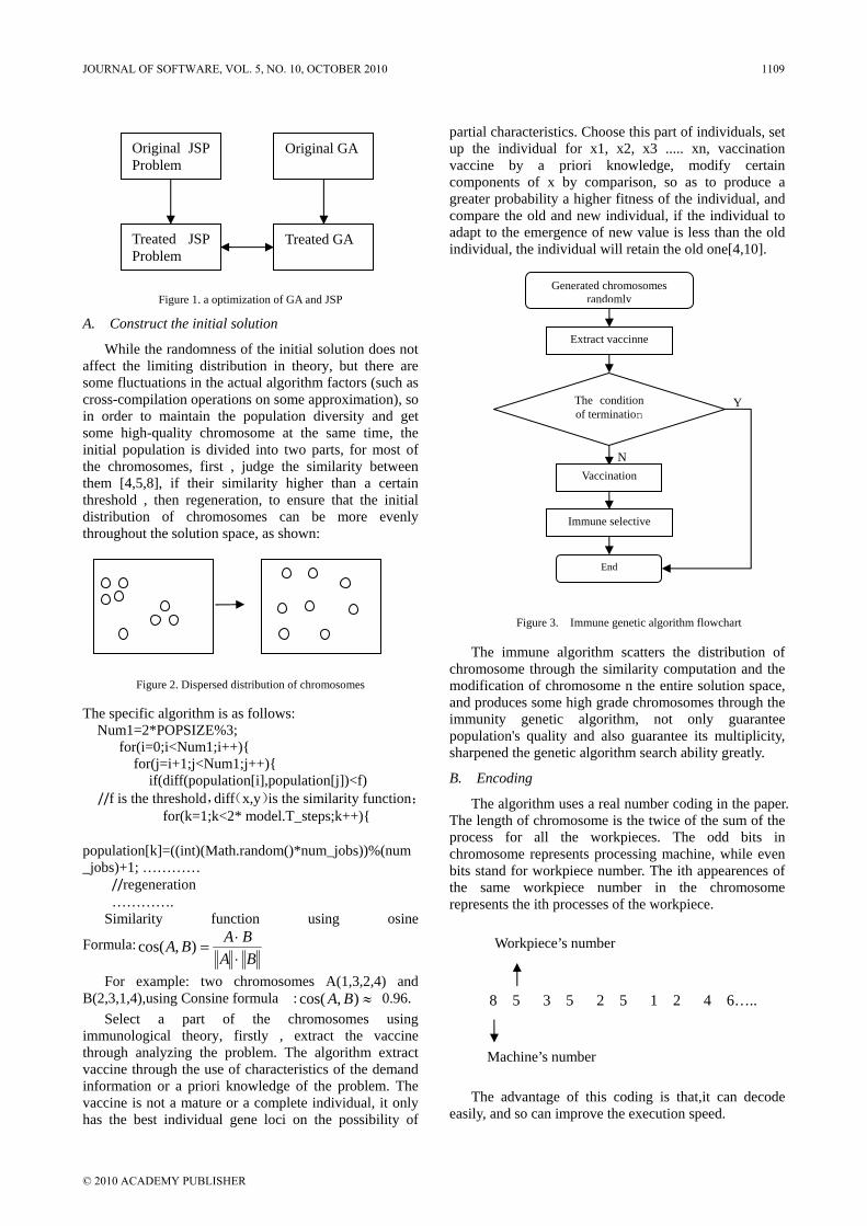
Figure 1. a optimization of GA and JSP

A. Construct the initial solution

While the randomness of the initial solution does not affect the limiting distribution in theory, but there are some fluctuations in the actual algorithm factors (such as cross-compilation operations on some approximation), so in order to maintain the population diversity and get some high-quality chromosome at the same time, the initial population is divided into two parts, for most of the chromosomes, first , judge the similarity between them [4,5,8], if their similarity higher than a certain threshold , then regeneration, to ensure that the initial distribution of chromosomes can be more evenly throughout the solution space, as shown:

Figure 2. Dispersed distribution of chromosomes

The specific algorithm is as follows:

Num1=2*POPSIZE%3; for(i=0;i<Num1;i++)

for(j=i+1;j<Num1;j++) if(diff(population[i],population[j])<f)

//f is the threshold，diff（x,y）is the similarity function； for(k=1;k<2* model.T_steps;k++)

population[k]=((int)(Math.random()*num_jobs))%(num_jobs)+1; …………

//regeneration ………….

Similarity function using osine

Formula:BA

BABA⋅⋅

=),cos(

For example: two chromosomes A(1,3,2,4) and B(2,3,1,4),using Consine formula : ≈),cos( BA 0.96.

Select a part of the chromosomes using immunological theory, firstly , extract the vaccine through analyzing the problem. The algorithm extract vaccine through the use of characteristics of the demand information or a priori knowledge of the problem. The vaccine is not a mature or a complete individual, it only has the best individual gene loci on the possibility of

partial characteristics. Choose this part of individuals, set up the individual for x1, x2, x3 ..... xn, vaccination vaccine by a priori knowledge, modify certain components of x by comparison, so as to produce a greater probability a higher fitness of the individual, and compare the old and new individual, if the individual to adapt to the emergence of new value is less than the old individual, the individual will retain the old one[4,10].

Figure 3. Immune genetic algorithm flowchart

The immune algorithm scatters the distribution of chromosome through the similarity computation and the modification of chromosome n the entire solution space, and produces some high grade chromosomes through the immunity genetic algorithm, not only guarantee population's quality and also guarantee its multiplicity, sharpened the genetic algorithm search ability greatly.

B. Encoding

The algorithm uses a real number coding in the paper. The length of chromosome is the twice of the sum of the process for all the workpieces. The odd bits in chromosome represents processing machine, while even bits stand for workpiece number. The ith appearences of the same workpiece number in the chromosome represents the ith processes of the workpiece.

The advantage of this coding is that,it can decode

easily, and so can improve the execution speed.

8 5 3 5 2 5 1 2 4 6…..

Workpiece’s number

Machine’s number

Original JSP Problem

Original GA

Treated JSP Problem

Treated GA

N

Y

Generated chromosomes randomly

Extract vaccinne

The condition of termination

Vaccination

Immune selective

End



C. Self-adapting crossover and mutation

a) Several concepts for probability of self-adapting crossover and mutation

In the GA, the limited space of all the individuals is Ω ,the entire solution space of all the populations corresponding is P, once the number and length of a given chromosome is identified, then Ω ,which is the

number of dimensions ofΩ is limited, and ΡN，the

number of dimensions of P is also limited. As the status of each generation in the algorithm only related with crossover, mutation and selection operation, but not related with algebra, so GA algorithm can be viewed as a finite state homogeneous Markov chain. The cross-state transition matrix decided by crossover operation is labeled by PPijcC ×= )( ,and ijc is defined as the

probability of cross-post from the state i to state j. while mutation operators determine the status of the transfer matrix PPijmM ×= )( , ijm is defined as the

probability of mutation from the state i to state j. and selection operation determine the status of the transfer matrix PPijsS ×= )( , ijs is defined as the

probability of selection from the state i to state j. The GA algorithm can be expressed as the following Markov chain:

1+= kk CMSPP

kP is the state of the kth generation. C is the cross-state transition matrix, M is mutation transfer matrix and S is selection transfer matrix. b) Design of adaptive crossover and mutation probability.

The important condition of Genetic algorithm convergence is to ensure that the optimal individual not to be destroyed or less destroyed, called the elitist strategy or a strategy for ensuring quality [6,7,9,12,14], in order to achieve this goal, we hope to give a lower crossover probability and mutation probability to chromosome with high adaptive value while higher crossover probability and mutation probability to chromosome with low adaptive value, so that in the evolutionary process the crossover can be eliminated as quickly as possible. Meanwhile, the adaptive crossover and mutation probability should be applied throughout the evolutionary process, At the start of the algorithm requires a relatively high probability of crossover and mutation in order to maintain population diversity, otherwise, in the initial stage, a number of individual with high adaptive value is difficult to cross with other individuals to exchange information. and genes of these outstanding individuals are difficult to be inherited and so resulted in premature convergence. In the final part of the algorithm requires a lower probability of crossover and mutation in order to expedite the convergence speed. In this paper we design crossover probability as follows:

⎪⎩

⎪⎨

⎧

<−−

>=

−

−

ffffffpffp

paiaic

kaic

k

i ),/()(

,

maxmaxηη

η is an adjustable constant, and between 1 and 1.02.and, if the algorithm converges too fast, then take a smaller number to slow down the speed of evolution, otherwise, take a bigger number to speed up the speed of evolution. K is the number of evolution. f i is the value

of individual fitness and f a is the value of average

fitness for the group. f max is the highest adaptive value

of the group. pc is the crossover probability.

Crossing method using partially mapping cross, first, randomly select two crossover points, exchange the fragments of parent individual between two cross-points,for the genes remaining, if they does not conflict with the fragments changed ,they will be kept, otherwise, determine the genes through the partially mapping, until there are non-conflict genes in individule, and obtain the individual offspring finally. For example, there are two parent individuals ]91|7358|264[

1=p ,

]93|1876|452[2=p , if the cross-point is 3,7, then the

fragment exchange. For the remaining genes, since Digital 2 does not conflicts with fragment (1876) ,keep digital 2, for digital 6, there is a conflict,and its mapping gene 8 are still conflicts, but for the digital 3 which is the mapping gene of digital 8, there is no conflict, it will be filled in the corresponding location of the child individual. Followed by analogy, we get the child individual ]95|1876|234[1 =c , we can also get the other

child individual ]96|7358|412[2=c similarly. This

operator meet the fundamental nature of the holland’s Schema Theorem in a certain extent, the child individuals inherit an effective model of the parent individuals.

At the same time,we add a small-scale competitive merit-based operation in a small scope In the crossover operation, if a pair of parent chromosomes A, B, cross-post them n times, resulting in 2n offspring individuals, choose the highest fitness value of individual offspring to join the offspring queue, repeat the above operations, until generate the specified number of offspring of individuals. At the same time, after adding small-scale competitive merit-based operation, the algorithm can avoid the "inbreeding", such as chromosomes X, Y generated the x, y by the cross operation, in the next round of genetic operation, x, y may be selected as the new parents to run cross operations, the algorithm convergence rate can be speeded up. c). Design of adaptive crossover operation

Mutation operator is just similar to the cross operator. The mutation operator design as follow:



⎪⎩

⎪⎨⎧

<−−

>=

−

−

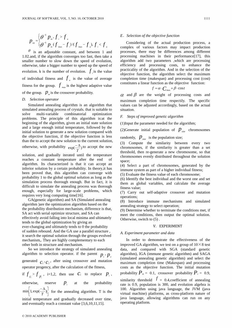
ffffffpffp

paiaim

kaim

k

mi ),/()(

,

maxmaxθθ

θ is an adjustable constant, and between 1 and 1.02.and, if the algorithm converges too fast, then take a smaller number to slow down the speed of evolution, otherwise, take a bigger number to speed up the speed of evolution. k is the number of evolution. f i is the value

of individual fitness and f a is the value of average

fitness for the group. f max is the highest adaptive value

of the group. pm is the crossover probability.

D. Selection operator Simulated annealing algorithm is an algorithm that

simulated annealing process of crystals. that is suitable to solve multi-variable combinatorial optimization problems. The principle of this algorithm is:at the beginning of the algorithm, given an initial state solution and a large enough initial temperature, followed by the initial solution to generate a new solution compared with the objective function, if the objective function is less than the to accept the new solution to the current solution, otherwise, with probability )exp(

T∆− to accept the new

solution, and gradually iterated until the temperature reaches a constant temperature after the end of algorithm. Its characterized is that it can accept an inferior solution by a certain probability. In theory,it has been proved that, this algorithm can converge with probability 1 to the global optimal solution as long as the simulation process thorough enough. But in fact, it is difficult to simulate the annealing process was thorough enough, especially for large-scale problems, which requires very long computing time[16].

GA(genetic algorithm) and SA (Simulated annealing algorithm )are the optimization algorithm based on the the probability distribution mechanism, difference is that, SA act with serial optimize structure, and SA can effectively avoid falling into local minima and ultimately tends to the global optimization by giving an ever-changing and ultimately tends to 0 the probability of sudden rebound. And the GA use a parallel structure , it search the optimal solution through the groups evolved mechanism,. They are highly complementary to each other both in structure and mechanism.

So we introduce the strategy of simulated annealing algorithm to selection operator. if the parent p1

, p2

generated c1, c2

, after using crossover and mutation operator progency, after the calculation of the fitness,

if ff pc ii

> , i=1,2, then use ci to replace pi ,

otherwise, reserve pi at the probability

⎥⎦⎤

⎢⎣⎡ ∆− )exp(,1min

T for the annealing algorithm. T is the

initial temperature and gradually decreased over time, and eventually reach a constant value [3,6,10,11,15].

E．Selection of the objective function

Considering of the actual production process, a complex of various factors may impact production processes, there may be differences among different processing machines in their performance[17], this algorithm add two parameters ,which are processing efficiency and processing costs, to enhance the practicality of the algorithm. And in the selection of the objective function, the algorithm select the maximum completion time (makespan) and processing cost (cost) constitutes a linear function as the objective function:

tf C cosmax ⋅+⋅= βα

α and β are the weight of processing costs and maximum completion time respectily. The specific values can be adjusted accordingly, based on the actual situation.

F. Steps of improved genetic algorithm

(1)Input the parameter needed for the algorithm;

(2)Generate initial population of psize chromosomes

randomly, psize is the population size; (3) Compute the similarity between every two chromosomes, if the similarity is greater than a set threshold, then re-generate a new chromosome, so that chromosomes evenly distributed throughout the solution space; (4) Select a part of chromosomes, generated by the immune system as part of a higher individual fitness; (5) Evaluate the fitness value of each chromosome; (6) Identify the best individual and the worst one and set them as global variables, and calculate the average fitness value; (7) Carry out self-adaptive crossover and mutation operations; (8) Introduce immune mechanisms and simulated annealing strategy to select operation; (9) Determine whether to terminate the conditions met, if meet the conditions, then output the optimal solution. Otherwise, switch to (5) .

V. EXPERIMENT

A. Experiment parameter and data

In order to demonstrate the effectiveness of the improved GA algorithm, we test on a group of 10×8 test data, and compared with SGA (standard genetic algorithm), IGA (immune genetic algorithm) and SAGA (simulated annealing genetic algorithm) and select the maximum completion time (Makespan) and processing costs as the objective function. The initial mutation probability Pm = 0.1, crossover probability Pc = 0.9,

similarity threshold f = 0.4,coefficient of annealing rate is 0.9, population is 300, and evolution algebra is 100. Algorithm using java language, the JVM (java virtual machine) platforms, as cross-platform nature of java language, allowing algorithms can run on any operating platform.



Figure 4. Algorithm flow chart

TABLE 1. Processing data

Process1(time) Process2 Process3Workpiece1 4 2 3 Workpiece2 5 1 8 Workpiece3 10 6 3 Workpiece4 3 4 5 Workpiece5 2 1 3 Workpiece6 1 4 5 Workpiece7 4 3 4 Workpiece8 9 2 7 Workpiece9 7 8 2 Workpiece10 8 2 7

TABLE 2. Performance of Machine Processing

Processing efficiency Processing costsMachine1 0.8 1 Machine2 0.7 2 Machine3 0.8 3 Machine4 0.8 2 Machine5 1.0 1 Machine6 0.8 2 Machine7 0.8 2 Machine8 1.0 1

Here, the weights of Processing cost and the maximum

completion time are α = 0.4 and β = 6.0 respectively.

B. Experiment result

We can abtain these result following after running SGA,IGA,GASA and IGASA respectively about 100 times:

TABLE 3. Operational Results

SGA IGA GASA IGASA

Optimum 240.71 238.85 238.45 232.23 Average 322.96 323.56 318.12 310.18

End Generation

41 52 55 65

Figure 5. Comparison of SGA,IGA,GASA and IGASA

As table 3 and figure 5 shows, we can see that in the comparison with other algorithms, the optimal value computed by our improved genetic algorithm is better than other algorithms. And the initial value of populations is better than others due to adding immue algorithm and judging similarity of different chromosomes. While adding the adaptive crossover and mutation probability and simulated annealing strategies, enabling the improved genetic algorithm can better search and can also be more effective to prevent "premature" phenomenon. The following table shows one of the optimal scheduling results:

N

Y

Input the parameter

Generate initial population

Dispersed distribution of chromosomes

Regenerator a part of chromosomes using immue system

Evaluate the fitness value of chromosomes

Identify the best individual and the worst one as global variables

Identify the best individual and the worst one as global variables

Carry out self-adaptive crossover and mutation operations

Carry out select operations with immune mechanisms and simulated annealing

strategy

Judge the terminate condition

end



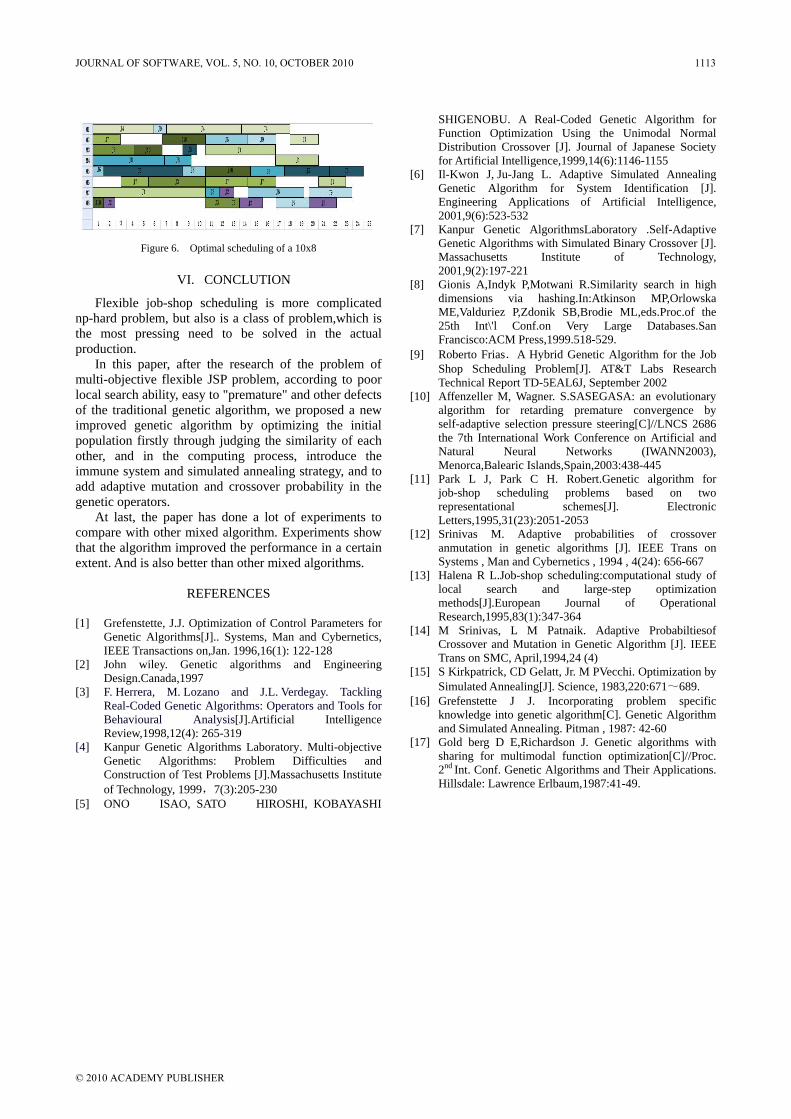
Figure 6. Optimal scheduling of a 10x8

VI. CONCLUTION

Flexible job-shop scheduling is more complicated np-hard problem, but also is a class of problem,which is the most pressing need to be solved in the actual production.

In this paper, after the research of the problem of multi-objective flexible JSP problem, according to poor local search ability, easy to "premature" and other defects of the traditional genetic algorithm, we proposed a new improved genetic algorithm by optimizing the initial population firstly through judging the similarity of each other, and in the computing process, introduce the immune system and simulated annealing strategy, and to add adaptive mutation and crossover probability in the genetic operators.

At last, the paper has done a lot of experiments to compare with other mixed algorithm. Experiments show that the algorithm improved the performance in a certain extent. And is also better than other mixed algorithms.

REFERENCES

[1] Grefenstette, J.J. Optimization of Control Parameters for

Genetic Algorithms[J].. Systems, Man and Cybernetics, IEEE Transactions on,Jan. 1996,16(1): 122-128

[2] John wiley. Genetic algorithms and Engineering Design.Canada,1997

[3] F. Herrera, M. Lozano and J.L. Verdegay. Tackling Real-Coded Genetic Algorithms: Operators and Tools for Behavioural Analysis[J].Artificial Intelligence Review,1998,12(4): 265-319

[4] Kanpur Genetic Algorithms Laboratory. Multi-objective Genetic Algorithms: Problem Difficulties and Construction of Test Problems [J].Massachusetts Institute of Technology, 1999，7(3):205-230

[5] ONO ISAO, SATO HIROSHI, KOBAYASHI

SHIGENOBU. A Real-Coded Genetic Algorithm for Function Optimization Using the Unimodal Normal Distribution Crossover [J]. Journal of Japanese Society for Artificial Intelligence,1999,14(6):1146-1155

[6] Il-Kwon J, Ju-Jang L. Adaptive Simulated Annealing Genetic Algorithm for System Identification [J]. Engineering Applications of Artificial Intelligence, 2001,9(6):523-532

[7] Kanpur Genetic AlgorithmsLaboratory .Self-Adaptive Genetic Algorithms with Simulated Binary Crossover [J]. Massachusetts Institute of Technology, 2001,9(2):197-221

[8] Gionis A,Indyk P,Motwani R.Similarity search in high dimensions via hashing.In:Atkinson MP,Orlowska ME,Valduriez P,Zdonik SB,Brodie ML,eds.Proc.of the 25th Int\'l Conf.on Very Large Databases.San Francisco:ACM Press,1999.518-529.

[9] Roberto Frias．A Hybrid Genetic Algorithm for the Job Shop Scheduling Problem[J]. AT&T Labs Research Technical Report TD-5EAL6J, September 2002

[10] Affenzeller M, Wagner. S.SASEGASA: an evolutionary algorithm for retarding premature convergence by self-adaptive selection pressure steering[C]//LNCS 2686 the 7th International Work Conference on Artificial and Natural Neural Networks (IWANN2003), Menorca,Balearic Islands,Spain,2003:438-445

[11] Park L J, Park C H. Robert.Genetic algorithm for job-shop scheduling problems based on two representational schemes[J]. Electronic Letters,1995,31(23):2051-2053

[12] Srinivas M. Adaptive probabilities of crossover anmutation in genetic algorithms [J]. IEEE Trans on Systems , Man and Cybernetics , 1994 , 4(24): 656-667

[13] Halena R L.Job-shop scheduling:computational study of local search and large-step optimization methods[J].European Journal of Operational Research,1995,83(1):347-364

[14] M Srinivas, L M Patnaik. Adaptive Probabiltiesof Crossover and Mutation in Genetic Algorithm [J]. IEEE Trans on SMC, April,1994,24 (4)

[15] S Kirkpatrick, CD Gelatt, Jr. M PVecchi. Optimization by Simulated Annealing[J]. Science, 1983,220:671～689.

[16] Grefenstette J J. Incorporating problem specific knowledge into genetic algorithm[C]. Genetic Algorithm and Simulated Annealing. Pitman , 1987: 42-60

[17] Gold berg D E,Richardson J. Genetic algorithms with sharing for multimodal function optimization[C]//Proc. 2nd Int. Conf. Genetic Algorithms and Their Applications. Hillsdale: Lawrence Erlbaum,1987:41-49.



Design and Implementation of Safety Expert Information Management System of Coal Mine

Based on Fault Tree WANG Cheng-gang

QingDao Technological University Computer Engineering Institute Qingdao,China [email protected] WANG Zi-zhen

DONGHUA University College of Information Science and Technology Sanghai, China

[email protected]

Abstract—Using the principle and method of fault tree and combining computer information system, the safety information closed-loop control system is formed with the characteristics of automatic control and automatic conversion. It has very important significance for coal mine safety to predict and deal with the hidden danger automatically, rapidly and timely. Based on this, we develop a safety information processing system according to fault tree of coal mine, which runs under the way of WEB. In this paper, we firstly introduce the overall structure and the component of the expert system, illustrate the fault tree analysis method in detail; then describe the key technologies and implementation method of software development and the program is given; finally, explain the important role of system implementation in solving the safety information management problem of coal mine.

Index Terms—Safety Information, Closed-loop Control, Expert System, Accident Tree, Workflow

I. INTRODUCTION

Coal is a high-risk industry, coal mine safety accidents caused heavy losses to enterprises, so reducing safety accidents become national great demand and the main task of coal enterprises. Facing the complex coal mine safety factor, we develop this project to control the hidden trouble of coal mine by safety management, and automatically predict accidents and controllable plans by expert system [1].

Current situation of information security management basically has the following questions:

A. The safety management is a complex dynamic system with various influence factors, information is processed mainly with artificial or record，needs long time to input information and print out report forms, a large number of hidden information cannot be tracked and supervised automatically.

B. he traditional mode is passive and lagging behind, lessons can be summed up only after the accident, can not analyze, evaluate and predict the potential danger existing in every production process, let alone to guide to adopt prevention plans and measures, eliminating hidden

dangers ahead of time. C. People can not analyze and evaluate the

equipment and environment rapidly before accident. Due to lack of scientific analysis and prediction, they can not timely judge the form, development and rigger conditions of accident.

With the development of computer technology and national attention to safety work, we already have the basis to development. Through the development of coal mine safety information expert system, the goal of the paper is to make a significant drop of major hidden danger and accidents and form a stable situation of production safety [2].

Accident tree is a kind of reliability analysis method which is firstly proposed by H A Walson of Bell laboratories. Fault Tree Analysis (FTA), also called Decision Tree, is a kind of method which ratiocinates the possible consequences by the initial event according to time sequence, thus identify the hazard source [3]. Mine accident is commonly the result of the successively occurrence of hidden danger, and some accidents happen with the occurrence of other hidden danger. There is a cause-and-effect logic relationship in the time and sequence of the hidden danger existence[4]. The situation is analyzed with tree diagram, so called fault tree. It can qualitatively understand the dynamic changes of the whole incident, and quantitatively compute the probability of each stage of development, in order to understand the process and state of the accident, and the probability of various states [5].

According to the principle of fault tree and the hidden danger examined every day, we analyze all stages step by step through time development and mutual relationship. On the basis of the possible subsequent events of each hidden danger, we select the two opposite states and find out the interrelated subsequent events. Then we analyze the safety or risk of these events, gradually advancing, until find out the major hidden dangers or the results of accidents [6]. If there is danger, indicate it and call out response plans for leadership and stuff to refer and make decision. The automatical workflow engine software of the computer will inform the relevant responsible persons, and keep tracking until the safety control personnel to review and verificate. The

WANG Cheng-gang（1963-）[email protected]



Figure 1: Overall structure of coal mine safety accident tree expert system

closed-loop control system of coal mine hidden dangers will be formed [7].

II. OVERALL DESIGN OF INFORMATION MANAGEMENT EXPERT SYSTEM OF COAL MINE SAFETY ACCIDENT TREE

Information management expert system of coal mine safety fault tree is a computer software system with automatic conversion of workflow as the center .After the collection of hidden danger information of three classes, based on the comprehensive use of expert experience and logic knowledge, we find out the eventually accident point and the cause of the accident by computer computing. If confirmed by control safety personnel, it will return to the relevant responsible persons, finally remove the hidden dangers automatically or artificially [8].

The framework of mine accident tree expert system contains nine parts: the automatic classifying information network platform based on computer network and workflow engine, the explaination institutions, the knowledge acquisition management institution, the dynamic database, the fault tree knowledge base, the inference engine, the evaluation optimizing institution, the self learning module and safety management and the safety management information system[9]. System structure is shown in figure 1.

The functions of each part are described as follows:

A. Computer network and workflow engine of automatic classifying information transmission platform

Taking the company’s LAN or INTERNET as platform, the coal mine safety information management system, which is based on workflow, automatically

transfers the security information to different role in the form of workflow. Operators can put the problems and hidden dangers forward through computer or short message, the system will answer them and output the results into computer or mobile phone. And when there is error between the results and the system, system can revise the parameters artificially form self learning mechanism according to experience through computer or short message [10].

B. System interpretation institutions.

The possible cause and result of accidents could be explained and reasonable solution will be provided, accident treatment plan will be provided to the accident with dangerous consequences. Interpretation system mainly explains the behavior and results to the user, how the reasoning result comes from.

C. Knowledge acquisition management institution.

The safety administrator, The professional management staff and security experts input the questions, the hidden dangers, the accident experience knowledge and logical knowledge through computer, deposit them to knowledge base in standardization form, and construct fault tree.

D. Dynamic database.

This database can store the known facts and intermediate results, and the real-time data and historical data of safety monitoring, ventilation, safety information management.



Table 1: The unsafe incidents

E. Knowledge base (fault tree).

It deposits safety rules, accident classification, characteristics, accident algorithm and reasoning rules, reflects cause-and-effect relationship of the system; we can be used for accident reasoning. Knowledge of knowledge base includes experience knowledge, logic knowledge and metaknowledge. Metaknowledge is knowledge about building, managing and operating the fault tree. Knowledge in knowledge base is organized in tree structure according to the representation, the nature, the level and the content of the knowledge.

F. Inference engine.

It is the knowledge reasoning components of the whole system. The inference is completed by computer reasoning algorithm, including two aspects as reasoning and control. A mixed mechanism combined with forward reasoning and backward reasoning is used in the system.

G. Evaluation optimizing institution. In the continuous operation of the system, correctness of the reasoning and problem solving ability can be improved by making continuously periodic evaluation to the reasoning process and the knowledge source. According to the user and state of system, the knowledge with bad predicting ability will be marked and stopped using. The lacking knowledge will be warned and prompted.

H. Self learning module.

According to the summary of system evaluation and action effects of control commands, it carries on correctness to the knowledge and instruction of the

system. Simultaneously, it can continually perfect and innovate the system, and enrich the knowledge in knowledge base real-timely, automatically revise and delete the knowledge which the system performance is weak and control deviation is strong. So the system can adapt to the coal mine’s complex safety condition and forecast exactly.

I. Coal mine safety management monitoring institution and information management system.

This organization mainly depends on the existing safety monitoring system and safety production management information system, takes the workflow engine as the platform. The information can be shared among each application system. Simultaneously hidden dangers and questions will be found through the prompting of inference organization and then automatic reduction ability can be achieved [11].

III. BASIC THEORY OF FAULT TREE ANALYSIS

Fault tree is the core of the whole knowledge base; it is made up of qualitative analysis and quantitative analysis. Qualitative analysis is to find the reasons and the reason combination of the top event. It can help us to redue the potential failure and modify the safety operation management plan. Quantitative analysis mainly calculates and estimates the probability of top event and the importance degree of bottom event. Through the qualitative analysis and quantitative analysis, effect of the factors of safety management is revealed, which have important meaning to improve the accuracy in safety management and the accident prevention [12].

A. Qualitative analysis



Figure 2: The gas explosion fault tree

The minimum cut sets and the minimum path sets play an important role in the qualitative analysis; the fault tree analysis will achieve maximum results with little effort if we apply the two methods flexibly. It will provide important basis to control accident effectively [11]. Because of the minimum path sets can be obtained by the minimum cut set, only minimum cut set is introduced here. The application of qualitative analytic method sees the following example.

B. Calculation of the top event’s probability There are several methods to calculate the occurrence

probability of top event, including two algorithms common used; the minimum cut set algorithm and the path minimum set algorithm. It is much simpler to use quantitative analysis method and the minimum cut set algorithm because there are many or-gate in the system. The minimum cut set includes logic "add" and "multiply", the probability function of fault tree can be written in the form of logic "multiply" of the minimum cut set [14].

1

( ) ( ) [1 (1 )]j

p

i ij i p

g q p T q= ∈

= = − −∏ ∏ (1)

Where, 1 2 ... ( 1,2,3,..., )i mp x x x i k= + + + = (2)

M is the number which the basic event jp contains. Calculate the probability of the top event of accident tree top according to including-excluding formula:

1

1 1 1

( ) 1 (1 ) (1 ) ... ( 1) (1 )j h j

p np

i i ir h j pi p i p p i

g q q q q−

= ≤ ≤∈ ∈ ∪ =

= − − + − + + − −∑ ∑∏ ∏ ∏p

(3)

Where, I is the ordinal number of the basic event; p is the number of the minimum path set; r, h, j is the ordinal number of the minimum path set.

C. Calculation of importance degrees The contribution of an element components or

minimum cut set made to the occurrence of the top event

is called importance degree. Due to the different design object, the calculation methods of importance degree are different, currently, the main means are the structure importance, the probability importance, the critical importance, the cut importance and the fuzzy importance developed in recent years [15]. The structure importance will be mainly introduced in this paper.

The structure importance is the important degree of the basic event analyzed from the structure of fault tree [16]. When the state of xi changes from 0 to 1 and the other basic state remains unchanged, the state of top

event changes from 0),0( =xiφ to 1),1( =xiφ , in other words, the basic event has played an important role to the top event, multiplies the accumulation of all these events by 1/2n-1 (“n” is the number of the basic event for the accident tree), we get the structure importance:

1

[ (1, ) ( 0 , ) ]( )

2 n

x xI i

φ φ−

−= ∑

(4)

IV. REALIZATION OF THE KEY TECHNOLOGIES OF THE SYSTEM

A. Establishment of Gas explosion Fault Tree and computation example

We rest on the New Coal Industry Group all previous years accident record file to carry on the analysis and statistics, choose the major accident as top event according to the principles for defining the top event, then seek all the direct factors which lead to the top event, and push down by the time until not constituting significant affecting factors. Figure 2 is the gas explosion fault tree. Table 1 is the unsafe incidents. a. Minimal cut set solution of the Fault tree

The minimal cut sets are congregation of elementary events of top event, is the hazards resource and way of accident occurrence, which has reflected system's risk. The goal of qualitative fault tree analysis is to find all minimal cut sets, discover the system hidden dangers or all possible causes of the appointed top event occurrence,



and systematically find out possible problems to cause the top event from the hidden danger inspection. In this paper, we use the method of Boolean algebra simplification to calculate all fault tree's minimal cut sets, the fault tree’s function structural equation is:

19 20 6 7 8 1 2 3 4 5

9 10 17 18

T=X X (X X X + X + X + X + X + X )(X + X +...+ X + X )

⋅

⋅ (5)

By simplifying we can see that the fault tree's minimal cut sets has 60, in sequence is:

1 19 20 6 7 8 9

2 19 20 6 7 8 10

3 19 20 6 7 8 11

10 19 20 6 7 8 18

11 19 20 1 9

20 19 20 1 18

51 19 20 5 18

K =X , X , X , X , X , X K =X , X , X , X , X , X K =X , X , X , X , X , X ...K =X , X , X , X , X , X K =X , X , X , X ...K =X , X , X , X ...K =X , X , X , X ...

60 19 20 5 18K =X , X , X , X

(6)

b. Structure importance analysis The contribution to top event occurrence which a

bottom event or the minimal cut set has is called the importance degree. The important degree analysis is playing a guidance role in reliability prediction and inspection in coal mine safety system, the systems operation and consummation, the formation of expert reserves. The structure importance refers to the impact of the degree which each basic event occurs to top event occurrence only from the structural analysis and without regard to the basic events’ occurrence probability. After qualitative fault tree analysis, we may determine the safety system's weak point, compute the fault tree structure importance coefficients and sort them, may know that the bottom event have the size of impact on top event , whose order is the order of system reliable effect. Analysis algorithms of importance are more, just like the structure importance, the probability importance, the critical importance and cut-sets importance as well as fuzzy importance which recently appears. We select the structure importance’s quadratic formulas to solve the importance coefficient, the formula is as follows:

( ) 111 (1 )

2 ji j

i nx k

Iφ −∈

= − −∏ (7)

In the formula, I )(iφ is the i-th bottom event's

structure importance coefficient; jk is the total number

of minimal cut sets; jn is total number of bottom event

in minimal cut sets jk which the i-th bottom event

belong to; ji kx ∈ says that the i-th bottom event

belongs to the j-th minimal cut set.

(1)Iφ =…= (5)Iφ = 104 1

11 (1 )2 −− − =0.737

(6)Iφ = (7)Iφ = (8)Iφ = 106 1

11 (1 )2 −− − =0.272

(9)Iφ = (10)Iφ =…= (17)Iφ =

(18)Iφ = 54 1 6 1

1 11 (1 ) (1 )2 2− −− − ⋅ − =0.503

(19)Iφ = (20)Iφ = 50 104 1 6 1

1 11 (1 ) (1 )2 2− −− − ⋅ −

=0.99908268 The sorting of structure importance coefficient of each

bottom event is as follows: (19) ( 20) (1) (5) (9 ) (10 )...I I I I I Iφ φ φ φ φ φ= = = =f f

(17 ) (18) (6 ) (7 ) (8)... I I I I Iφ φ φ φ φ= = = = =f

B. The instance of the establishment of the workflow engine

The workflow engine is the critical part in entire system. The relevant personnel may track the workflow information by the level distribution in accordance with the order of management flow, and all levels of personnel sign and feedback the information to the senior leader after receiving the program information of the project. Through it the leadership can fully monitor the project flow[16].

We use the flow of issues notice to illustrate the setup procedure of workflow. As shown in Figure 2, process is as follows: First fill in the issues notice according to the problem which the inspectors check, sent to the work captain to carry on the inspection, and make the rectify notice by the safety inspectors senior, the process result is sent to safety supervision department to examines and approves, if reexamination is eligible, this flow end, otherwise, carrying on the penalties of individual integral, then fill in reexamination notice and orders rectification again, then enters the flow, until the entire department flow finishes [17]. Issues notice workflow is shown in Figure 3.

Process flow of issues notice W=（A，T，F，S，ID）, where,

A=a1,a2,a3,a4,a5 T= i,c1,c2,c3,c4,o c1=(I1,N1,F1,L1,D1,R1,S1) Vicissitude= (rule number, name, rule type, trigger

identification, executive conditions, executive actions, priority)

I1= No.1 N1: issues notice F1:Accept_Order(issues notice) L1:Null D1:(order ， orderName ， Re_OrderID ，

CreditID) R1:R11,R12 R11:(ON(EndOf(Assign))

IF(TRUE)DO(Accept_Order))



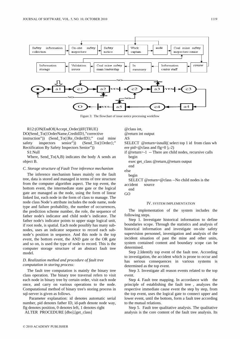
Figure 3: The flowchart of issue notice processing workflow

R12:(ON(EndOf(Accept_Order))IF(TRUE) DO(Send_To(OrderName,CreditID,”corrective instruction”)) (Send_To(Re_OrderID;” coal mine safety inspectors senior”)) (Send_To(Order;” Rectification By Safety Inspectors Senior”))

S1:Null Where, Send_To(A,B) indicates the body A sends an

object B.

C. Storage structure of Fault Tree inference mechanism The inference mechanism bases mainly on the fault

tree, data is stored and managed in terms of tree structure from the computer algorithm aspect. The top event, the bottom event, the intermediate state gate or the logical gate are managed as the node, using the form of linear linked list, each node in the form of class to manage. The node class Node’s attribute includes the node name, node type and failure probability, the number of occurrences, the prediction scheme number, the role, the sequence of father node's indicator and child node’s indicator. The father node's indicator points to upper stage logical unit, if root node, is spatial. Each node possibly has many sub-nodes, uses an indicator sequence to record each sub-node’s position in sequence. And this node is the top event, the bottom event, the AND gate or the OR gate and so on, is used the type of node to record. This is the computer storage structure of an abstract fault tree model.

D. Realization method and procedure of fault tree computation in storing process:

The fault tree computation is mainly the binary tree class operation. The binary tree traversal refers to visit each node in binary tree by certain order, visit each node once, and carry on various operations to the node. Computational method of binary tree's storing process in sql-server is given as follows.

Parameter explanation: id denotes automatic serial number, pid denotes father ID, id-path denote node way, flg denotes position, 0 denotes left, 1 denotes right ALTER PROCEDURE [dbo].[get_class]

@class int, @return int output AS SELECT @return=isnull(( select top 1 id from class where pid=@class and flg=0 ),-2) if @return>-1 -- There are child nodes, recursive calls begin exec get_class @return,@return output end else begin SELECT @return=@class --No child nodes is the accident source end GO

IV. SYSTEM IMPLEMENTATION

The implementation of the system includes the following steps.

Step 1. Investigate historical information to define boundaries scope. Through the statistics and analysis of historical information and investigate on-site safety supervision personnel, investigation and analysis of the incident situation of past the mine and other units, system contained content and boundary scope can be determined.

Step 2.Identify top event of the fault tree. According to investigation, the accident which is prone to occur and has serious consequences in various systems is determined as the top event.

Step 3. Investigate all reason events related to the top event.

Step 4. Fault tree mapping. In accordance with the principle of establishing the fault tree , analyzes the respective immediate cause event the step by step, from the top event, uses the logical gate to connect upper and lower event, until the bottom, form a fault tree according to the mutual relations.

Step 5. Fault tree qualitative analysis. The qualitative analysis is the core content of the fault tree analysis. Its



goal is to analyze the types of accident's occurrence rule and characteristic, find out a feasible plan to control the accident by striking a minimal cut set (or minimal path set), and analyze each basic event's important procedure from the accident structure and occurred probabilistic, in order to respectively take countermeasure in order of priority.

Step 6. Fault tree quantitative analysis. The task of quantitative analysis is to calculate and estimate the probability of the top event occurrence and bottom event's importance degree and so on.

Step 7. Learning system design. Form the perfect and applied security information specialist management system through the learning system to improve measures unceasingly.

V. CONCLUSIONS

A coal mine security information management expert system based on the fault tree is proposed, taken a variety of factors into consideration, The system improves through self-learning institutions with the fault tree's procedure. which is helpful to the safety managers to understand a variety of complex factors to control mine safety, discover the accident phenomenon as early as possible, definite the various causes of the accident, prevent the occurrence of accident and reduce serious damage of accident promptly[19]. It has strong science rigorous and versatility and high practical application value. At present this system is put into use in Zibo mining industry group and Xu Chang coal plants in China. The system is running well and realized automated analysis and automatic transmission of the security information. It innovatively changes the past form of coal mine safety management, enhances effectiveness and accuracy of safety in production, and improves coal mine's management level and economic efficiency greatly.

REFERENCES

[1] FAN Weitang, LU Jianzhang, SHEN Baohong. Technology and measures of mine hazards control[M]．Xuzhou: China University Mining and Technology Press, 2007.

[2] LIN Boquan, ZHOU Yan, LIU Zhen tang．Safety system engineering[M]．Xuzhou: China University Mining and Technology Press, 2005.

[3] Fitzgeerald R W.Building ． Fire safety evaluation method[R].Worcester Polytechnic Institute, 1993

[4] Watts JR, M John. Fire Safety Science[C].5th International Symposium, USA, 1997: 101-109

[5] Blaschke Wieslaw; Gawlik, Lidia. Coal mining industry restructuring in Poland: implications for the domestic and international coal markets. Applied Energy Volume: 64, Issue: 1-4, September 1, 1999, pp. 453-456

[6] Greb, Stephen F.; Popp, John T. Mining geology of the Pond Creek seam, Pikeville Formation, Middle Pennsylvanian, in part of the Eastern Kentucky Coal Field, USA. International Journal of Coal Geology Volume: 41, Issue: 1-2, August, 1999, pp. 25～50

[7] WFMC.Workflow Management Coalition Specification: Terminology & Glossary. Document Number WFMC-TC-1011, Brussels, 1996

[8] Petra H, Stefan J, Jens N, Katrin S, Michael T.A comprehensive approach to flexibility in workflow management systems[J].In: Software Engineering Notes, 1999

[9] Workflow Handbook [Z].Lighthouse Point, FL, USA: Future Strategies Inc., 2004

[10] LING Biaocan. Discussion on content of safety assessment for colliery flood [J].China Safety Science Journal, 2004, 14(7): 64-66.

[11] CAO Shugang, ZHANG Liqiang, LIU Yanbao, et al.Causing model of accidents and preventing system of small mines[j] .Journal of China Coal Society, 2008, 33(6): 629-634.

[12] LOU Chunhong, XIE Xianping.Comparison study of accident-causing theories [J] .Journal of Safety Science and Technology, 2007, 3(5): 111-115.

[13] JI Changwei, RONG Jili, HUANG Wenhu.Research on intelligent diagnosis for spacecraft based on fault tree and neural network [J] .Chinese Journal of Space Science, 1999, 19(2): 160-166.

[14] QIAN Xinming, CHEN Baozhi.Catastrophe model for accident cause [J] .China Safety Science Journal, 1995, 5(2): 1-4.

[15] YUAN Changming.On funding versatile solution of the least cut set and least path set in fault tree analysis by computer [J] .Journal of China Institute of Metrology, 2002, 13(4): 308-310.

[16] DING Caihong, HUANG Wenhu, JIANG Xingwei.A method of fault isolation for spacecraft based on minimum cut sets’ rank[J] .Chinese Journal of Space Science, 2000, 20(1): 89-94.

[17] MU Zhansheng, ZHOU Yun. The design and implementation of - distributed workflow system based on web service [J], Computer Application and Software, 2008 25(12): 99-101

[18] WANG Xianghui, WANG Kangjin. Embedded workflow system integration research [J], Computer Application and Software, 2008 25(11) 95-122

[19] Greb, Stephen F.; Popp, John T..Mining geology of the Pond Creek seam, Pikeville Formation, Middle Pennsylvanian, in part of the Eastern Kentucky Coal Field, USA. International Journal of Coal Geology Volume: 41, Issue: 1-2, August, 1999, pp. 25-50



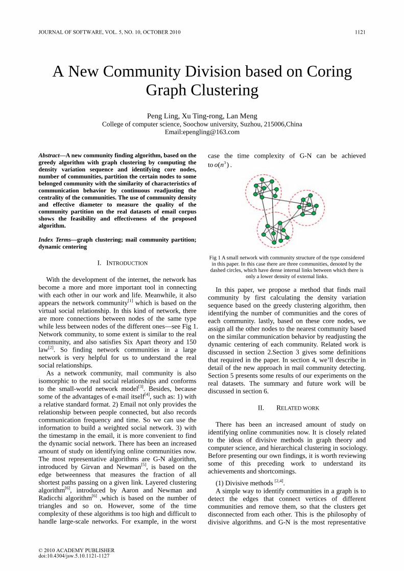
A New Community Division based on Coring Graph Clustering

Peng Ling, Xu Ting-rong, Lan Meng

College of computer science, Soochow university, Suzhou, 215006,China Email:[email protected]

Abstract—A new community finding algorithm, based on the greedy algorithm with graph clustering by computing the density variation sequence and identifying core nodes, number of communities, partition the certain nodes to some belonged community with the similarity of characteristics of communication behavior by continuous readjusting the centrality of the communities. The use of community density and effective diameter to measure the quality of the community partition on the real datasets of email corpus shows the feasibility and effectiveness of the proposed algorithm. Index Terms—graph clustering; mail community partition; dynamic centering

I. INTRODUCTION

With the development of the internet, the network has become a more and more important tool in connecting with each other in our work and life. Meanwhile, it also appears the network community[1] which is based on the virtual social relationship. In this kind of network, there are more connections between nodes of the same type while less between nodes of the different ones—see Fig 1. Network community, to some extent is similar to the real community, and also satisfies Six Apart theory and 150 law[2]. So finding network communities in a large network is very helpful for us to understand the real social relationships.

As a network community, mail community is also isomorphic to the real social relationships and conforms to the small-world network model[3]. Besides, because some of the advantages of e-mail itself[4], such as: 1) with a relative standard format. 2) Email not only provides the relationship between people connected, but also records communication frequency and time. So we can use the information to build a weighted social network. 3) with the timestamp in the email, it is more convenient to find the dynamic social network. There has been an increased amount of study on identifying online communities now. The most representative algorithms are G-N algorithm, introduced by Girvan and Newman[5], is based on the edge betweenness that measures the fraction of all shortest paths passing on a given link. Layered clustering algorithm[6], introduced by Aaron and Newman and Radicchi algorithm[6] ,which is based on the number of triangles and so on. However, some of the time complexity of these algorithms is too high and difficult to handle large-scale networks. For example, in the worst

case the time complexity of G-N can be achieved to 3( )o n .

Fig 1 A small network with community structure of the type considered in this paper. In this case there are three communities, denoted by the

dashed circles, which have dense internal links between which there is only a lower density of external links.

In this paper, we propose a method that finds mail

community by first calculating the density variation sequence based on the greedy clustering algorithm, then identifying the number of communities and the cores of each community. lastly, based on these core nodes, we assign all the other nodes to the nearest community based on the similar communication behavior by readjusting the dynamic centering of each community. Related work is discussed in section 2.Section 3 gives some definitions that required in the paper. In section 4, we’ll describe in detail of the new approach in mail community detecting. Section 5 presents some results of our experiments on the real datasets. The summary and future work will be discussed in section 6.

II. RELATED WORK

There has been an increased amount of study on identifying online communities now. It is closely related to the ideas of divisive methods in graph theory and computer science, and hierarchical clustering in sociology. Before presenting our own findings, it is worth reviewing some of this preceding work to understand its achievements and shortcomings.

(1) Divisive methods [2,4]. A simple way to identify communities in a graph is to

detect the edges that connect vertices of different communities and remove them, so that the clusters get disconnected from each other. This is the philosophy of divisive algorithms. and G-N is the most representative



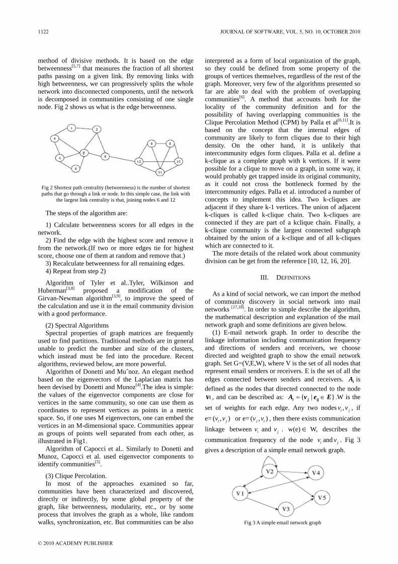
method of divisive methods. It is based on the edge betweenness[5,7] that measures the fraction of all shortest paths passing on a given link. By removing links with high betweenness, we can progressively splits the whole network into disconnected components, until the network is decomposed in communities consisting of one single node. Fig 2 shows us what is the edge betweenness.

Fig 2 Shortest path centrality (betweenness) is the number of shortest paths that go through a link or node. In this simple case, the link with

the largest link centrality is that, joining nodes 6 and 12

The steps of the algorithm are:

1) Calculate betweenness scores for all edges in the network.

2) Find the edge with the highest score and remove it from the network.(If two or more edges tie for highest score, choose one of them at random and remove that.)

3) Recalculate betweenness for all remaining edges. 4) Repeat from step 2)

Algorithm of Tyler et al..Tyler, Wilkinson and Huberman[3,8] proposed a modification of the Girvan-Newman algorithm[3,9], to improve the speed of the calculation and use it in the email community division with a good performance.

(2) Spectral Algorithms Spectral properties of graph matrices are frequently

used to find partitions. Traditional methods are in general unable to predict the number and size of the clusters, which instead must be fed into the procedure. Recent algorithms, reviewed below, are more powerful.

Algorithm of Donetti and Mu˜noz. An elegant method based on the eigenvectors of the Laplacian matrix has been devised by Donetti and Munoz[4].The idea is simple: the values of the eigenvector components are close for vertices in the same community, so one can use them as coordinates to represent vertices as points in a metric space. So, if one uses M eigenvectors, one can embed the vertices in an M-dimensional space. Communities appear as groups of points well separated from each other, as illustrated in Fig1.

Algorithm of Capocci et al.. Similarly to Donetti and Munoz, Capocci et al. used eigenvector components to identify communities[5].

(3) Clique Percolation. In most of the approaches examined so far,

communities have been characterized and discovered, directly or indirectly, by some global property of the graph, like betweenness, modularity, etc., or by some process that involves the graph as a whole, like random walks, synchronization, etc. But communities can be also

interpreted as a form of local organization of the graph, so they could be defined from some property of the groups of vertices themselves, regardless of the rest of the graph. Moreover, very few of the algorithms presented so far are able to deal with the problem of overlapping communities[6]. A method that accounts both for the locality of the community definition and for the possibility of having overlapping communities is the Clique Percolation Method (CPM) by Palla et al[6,11].It is based on the concept that the internal edges of community are likely to form cliques due to their high density. On the other hand, it is unlikely that intercommunity edges form cliques. Palla et al. define a k-clique as a complete graph with k vertices. If it were possible for a clique to move on a graph, in some way, it would probably get trapped inside its original community, as it could not cross the bottleneck formed by the intercommunity edges. Palla et al. introduced a number of concepts to implement this idea. Two k-cliques are adjacent if they share k-1 vertices. The union of adjacent k-cliques is called k-clique chain. Two k-cliques are connected if they are part of a kclique chain. Finally, a k-clique community is the largest connected subgraph obtained by the union of a k-clique and of all k-cliques which are connected to it.

The more details of the related work about community division can be get from the reference [10, 12, 16, 20].

III. DEFINITIONS

As a kind of social network, we can import the method of community discovery in social network into mail networks [17,18]. In order to simple describe the algorithm, the mathematical description and explanation of the mail network graph and some definitions are given below.

(1) E-mail network graph. In order to describe the linkage information including communication frequency and directions of senders and receivers, we choose directed and weighted graph to show the email network graph. Set G=(V,E,W), where V is the set of all nodes that represent email senders or receivers. E is the set of all the edges connected between senders and receivers. iA is defined as the nodes that directed connected to the node

iv , and can be described as: | = ∈i j ijA v e E .W is the set of weights for each edge. Any two nodes ,i jv v , if e= ( , )i jv v or e= ( , )j iv v , then there exists communication linkage between iv and jv . w(e) ∈ W, describes the communication frequency of the node iv and jv . Fig 3 gives a description of a simple email network graph.

Fig 3 A simple email network graph



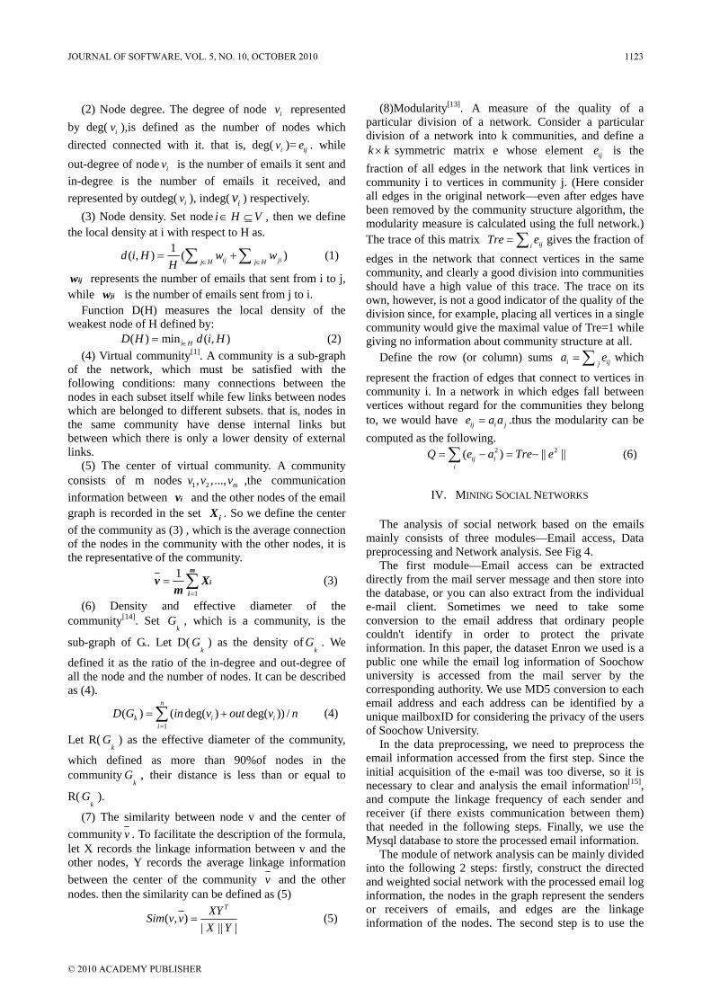
(2) Node degree. The degree of node iv represented by deg( iv ),is defined as the number of nodes which directed connected with it. that is, deg( iv )= ije . while out-degree of node iv is the number of emails it sent and in-degree is the number of emails it received, and represented by outdeg( iv ), indeg( iv ) respectively.

(3) Node density. Set node i H V∈ ⊆ , then we define the local density at i with respect to H as.

1( , ) ( )ij jij H j Hd i H w w

H ∈ ∈= +∑ ∑ (1)

ijw represents the number of emails that sent from i to j, while jiw is the number of emails sent from j to i.

Function D(H) measures the local density of the weakest node of H defined by:

( ) min ( , )i HD H d i H∈= (2) (4) Virtual community[1]. A community is a sub-graph

of the network, which must be satisfied with the following conditions: many connections between the nodes in each subset itself while few links between nodes which are belonged to different subsets. that is, nodes in the same community have dense internal links but between which there is only a lower density of external links.

(5) The center of virtual community. A community consists of m nodes 1 2, ,..., mv v v ,the communication information between iv and the other nodes of the email graph is recorded in the set iX . So we define the center of the community as (3) , which is the average connection of the nodes in the community with the other nodes, it is the representative of the community.

1

1=

= ∑m

ii

v Xm

(3)

(6) Density and effective diameter of the community[14]. Set

kG , which is a community, is the

sub-graph of G.. Let D(k

G ) as the density ofk

G . We

defined it as the ratio of the in-degree and out-degree of all the node and the number of nodes. It can be described as (4).

1( ) ( deg( ) deg( )) /

n

k i ii

D G in v out v n=

= +∑ (4)

Let R(k

G ) as the effective diameter of the community,

which defined as more than 90%of nodes in the community

kG , their distance is less than or equal to

R(k

G ).

(7) The similarity between node v and the center of community v . To facilitate the description of the formula, let X records the linkage information between v and the other nodes, Y records the average linkage information between the center of the community v and the other nodes. then the similarity can be defined as (5)

( , )| || |

TXYSim v vX Y

= (5)

(8)Modularity[13]. A measure of the quality of a particular division of a network. Consider a particular division of a network into k communities, and define a k k× symmetric matrix e whose element ije is the fraction of all edges in the network that link vertices in community i to vertices in community j. (Here consider all edges in the original network—even after edges have been removed by the community structure algorithm, the modularity measure is calculated using the full network.) The trace of this matrix iji

Tre e= ∑ gives the fraction of edges in the network that connect vertices in the same community, and clearly a good division into communities should have a high value of this trace. The trace on its own, however, is not a good indicator of the quality of the division since, for example, placing all vertices in a single community would give the maximal value of Tre=1 while giving no information about community structure at all.

Define the row (or column) sums i ijja e= ∑ which

represent the fraction of edges that connect to vertices in community i. In a network in which edges fall between vertices without regard for the communities they belong to, we would have ij i je a a= .thus the modularity can be computed as the following.

2 2( ) || ||ij ii

Q e a Tre e= − = −∑ (6)

IV. MINING SOCIAL NETWORKS

The analysis of social network based on the emails mainly consists of three modules—Email access, Data preprocessing and Network analysis. See Fig 4.

The first module—Email access can be extracted directly from the mail server message and then store into the database, or you can also extract from the individual e-mail client. Sometimes we need to take some conversion to the email address that ordinary people couldn't identify in order to protect the private information. In this paper, the dataset Enron we used is a public one while the email log information of Soochow university is accessed from the mail server by the corresponding authority. We use MD5 conversion to each email address and each address can be identified by a unique mailboxID for considering the privacy of the users of Soochow University.

In the data preprocessing, we need to preprocess the email information accessed from the first step. Since the initial acquisition of the e-mail was too diverse, so it is necessary to clear and analysis the email information[15], and compute the linkage frequency of each sender and receiver (if there exists communication between them) that needed in the following steps. Finally, we use the Mysql database to store the processed email information.

The module of network analysis can be mainly divided into the following 2 steps: firstly, construct the directed and weighted social network with the processed email log information, the nodes in the graph represent the senders or receivers of emails, and edges are the linkage information of the nodes. The second step is to use the



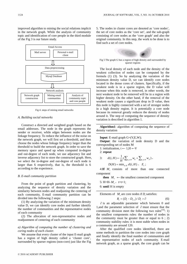
improved algorithm to mining the social relations implicit in the network graph. While the analysis of community topic and identification of core people in the third module of the Fig 3 is our future study.

Fig 4. steps of mining email networks

A. Building social networks

Construct a directed and weighted graph based on the email addresses. The node in the graph represents the sender or receiver, while edges between nodes are the linkage frequency. To reduce the influence of the noise on the network graph, we will first set a threshold, and then choose the nodes whose linkage frequency larger than the threshold to build the network graph. In order to save the memory space and speed up when computed in-degree and out-degree of each node, we use adjacency list and inverse adjacency list to store the constructed graph. Here, we select the in-degree and out-degree of each node is larger than 6 respectively, that is, the threshold is 6 according to the experience.

B. E-mail community partition

From the point of graph partition and clustering, by analyzing the sequence of density variation and the similarity between nodes and readjusting the centering of each community, E-mail community partition can be divided into the following 2 steps:

(1) By analyzing the variation of the minimum density value D, we can identify core nodes and further identify the number of communities and the representative nodes of each community

(2) The allocation of non-representative nodes and readjustment of centering of each community a) Algorithm of computing the number of clustering and coring nodes of each cluster.

We assume that every cluster of the input E-mail graph has a region of high density called a ‘cluster core’, surrounded by sparser regions (non-core) just like the Fig

5. The nodes in cluster cores are denoted as ‘core nodes’, the set of core nodes as the ‘core set’, and the sub-graph consisting of core nodes as the ‘core graph’ and also the original community. In this step, the work to be done is to find such a set of core nodes.

Fig 5 The graph G has a region of high density and surrounded by

sparser regions

The local density of each node and the density of the weakest collection of nodes can be computed by the formula (1) (3). So by analyzing the variation of the minimum density value D, we can identify core nodes located in the dense cores of clusters. Specifically, if the weakest node is in a sparse region, the D value will increase when this node is removed, in other words, the next weakest node to be removed will be in a region with higher density. On the other hand, if the removal of the weakest node causes a significant drop in D value, then this node is highly connected with a set of stronger nodes in a high density region. It is potentially a core node because its removal greatly reduces the density of nodes around it. The step of computing the sequence of density variation is described in algorithm 1.

Algorithm1: algorithm of computing the sequence of

density variation

Input: E-mail graph G=(V,E,W); Output: the variation of node density D and the

corresponding set of nodes M 1: initialization, t ← 1,H ←V 2: repeat

3: 1( , ) ( )ij jij H j Hd i H w w

H ∈ ∈= +∑ ∑ ，

( ) min ( , )i HD H d i H∈= ， cE ; 4:If tM consists of more than one connected

component then tM ← the smallest connected component 5: H=H- tM ，t=t+1; 6: until H is empty

Elements of tM are core nodes if tD satisfies:

1( ) /t t t tR D D D+= − > ∂ (6) ∂ is an adjustable parameter which between 0 and

1,and the parameter selection of ∂ must ensure that the community division meet the following two rules[10]: 1) the smallest components rules: the number of nodes in the community must be greater than or equal to 6 ; 2) community stability rules: it is most stable when nodes in a community are around 120.

After the qualified core nodes identified, there are some methods to partition the core nodes into core graph and finally identify the final number of communities and the representative nodes of each community. E-mail network graph, as a sparse graph, the core graph can be

Email Access

Mail server Personal e-mail client

Data preprocessing

Mysql Database

Network analysis

Network graph construction

Mining email communities

Analysis of community topic and core people



found from the connected components, and each component is considered as a cluster core or the representative nodes of the core graph—see Fig 6.

Fig 6. A sparse netwok including 3 core graphs.

b) community partition

After computing the number of clustering and coring nodes of each cluster, now we will discuss the community partition. Algorithm 2 described the steps of E-mail network community partition.

Algorithm 2: ENCD（Email Network Community

Detecting）E-mail network community partition Input: G=(V,E,W) Output: Community ID and the nodes of each

community 1: input the number of core graph K and core nodes of

each core graph computed by 2.2.1; 2: repeat 3: for t=(T,T-1,…,2,1) 4: for (centering of each of community) //find the

centering of community jc which is the greatest similar to tM

5: if tM includes non-core nodes labeled ix , then compute the similarity between ix and jc ,if sim( ix , jc )>= β ,then the community ID of ix is j and add the node into community jc //threshold β helps consider the situation that one node belongs to multi-communities

6: for each community community[j] 7: readjust the centering of the community[j]

//computed by formula (3) 8: util the centering of each community not change

again.

V. EXPERIMENT OF COMMUNITY PARTITION ON THE REAL DATASETS

We demonstrate the performance of our algorithm on the Enron email corpus and the email log information of Soochow university between February 2009 and May. The Enron email corpus is a set of emails belonging to 151 users, and consists of 252,759 email messages, it is now about a public network analysis corpus. which can be obtained from http://www-2.cs.cmu.edu/~enron/. Email log information of Soochow university(ELIS) included 183,925 nodes and 391,347 edges after processing, which including the communication

information of intramural mailboxes and extramural mailboxes. Considering the influence of the noise, after selecting the in-degree and out-degree of each node larger than 6 respectively, Email log information of Soochow university(ELIS) included only 5948 nodes and 23,479.

In the experiment, we took MD5 [19]conversion to each email address(mailbox) and each mailbox can be identified by a unique mailboxID for considering the privacy of the users of Soochow university.

Experiment environment: 2.80GHz Pentium CPU, 1G RAM, 80 GB hard drive; OS: Microsoft Windows XP; development platform :Myeclipse. The results of community partition are composed by mailboxID, which represents each mailbox, and communityID, which stands for the community labeling.

Fig 7 is the Visualization of the whole Enron Email graph. It constructs a social network. Fig 8 is the visualization of the community 6 computed by G-N on Enron, and the detail information of the community is depicted in Table II. Fig 9 is the visualization of the community 3 computed by ENCD on Enron, and the detail information of the community is depicted in Table III. We can see that either partition method, nodes in the same community are connected densely while between are much looser.

Fig 10 shows the results of community partition of Enron with different values of ∂ . We can see that the number of communities is quite similar although with different ∂ , So the influence of ∂ on the final results of community partition is not great.

Table I shows comparison of the results on Enron email corpus and email log information of Soochow University computed by our algorithm ENCD and G-N algorithm. Here ∂ =0.26 for the Enron and 0.125 for the email log information of Soochow university, modularity is one of the indicators for the evaluation of algorithms, usually it is a decimal between 0 and 1, and the greater the modularity is, the higher the quality of that community partition is. Its definition can be seen from the formula (6).

Table I

Comparison of the results computed by ENCD and G-N on the same datasets

algorithm dataset modularity Number of

communities

G-N Enron 0.372 8 ELIS 0.296 47

ENCD Enron 0.369 9 ELIS 0.301 50

Table II and III show the details about the results of

community partition of Enron computed by G-N and ENCD algorithm respectively.

From the table II and III, we can see that the results computed by G-N and ENCD are similar. But the distribution of the nodes in each community is of some difference. For example, there is only one node in the three communities computed by G-N algorithm and only two nodes in another on Enron while the distribution of



nodes computed by ENCD is mode even. So community partition of our algorithm on Enron is more natural and stable.

Table II

The detailed results computed by G-N algorithm on Enron

Community ID Nodes in the community

Community 1

146,37,80,71,96,90,41,127,112,122,61,44,8,101,145,117,128,56,26,1,139,148,40,17,24,59,125,77,104,100,62,107,140,38,10,126,91,118,103,108,105,106,120,81,73,25,150,111,58,69,129,49,92,54,83,78,84,47,34,110,114,151,51,95,39,113,124,22,88,

45,46,64,109,89,63,36,123,119,121,82,42,60,5 Community 2 2,3,4,18,19,20,28,29,30,32,55,66,68,72,74,137,14

1 Community 3 6,7,9,11,12,13,14,16,23,27,48,50,52,57,65,67,75,7

6,98,136,142,147 Community 4 33 Community 5 79 Community 6 15,85,86,87,93,97,99,115,130,131,132,133,134,13

5,138,143,149 Community 7 31,35 Community 8 43

Table III

The detailed results computed by ENCD algorithm on Enron

Community ID Nodes in the community

Community 1

2,3,4,6,9,13,16,18,19,20,23,27,28, 29,30,32,44,48,49,50,52,55,57,65 66,67,68,69,70,72,74,91,102,111 136,137,139,140,141

Community 2 10,17,21,25,26,36,37,58,75,77, 80 90,101,112,118,125,127,142

Community 3 85,86,87,97,99,115,130,131,133,134 135,149

Community 4 24,79,83,88,103,105,107,109,114,117 119,123,126,151

Community 5 7,11,12,33,38,76,98,147 Community 6 5,14,15,22,51,73,81,89,108,121,138,

143 Community 7 54,78,84,92,100,122,129 Community 8 31,34,35,39,43,45,82,94, 113,124 Community 9 1,8,40,41,42,46,47,56,59,60,61,62,63

64,71,93,95,96,104,106,110,120,128 132,145,146,148,150

Fig 11 describes the community density of Enron

computed by ENCD and G-N algorithm. Fig 12 is a description of the community effective diameter comparison on Enron by the two algorithms.

From the table I, II, III, we can see that the number of communities computed by ENCD on Enron email corpus is close to that of G-N, while nodes belonged to communities computed by G-N are not distributed average and even exists only one node in 2 communities and 2 nodes in another community which is conflicted with rule1, but results of ENCD are relatively average. Fig 5 shows that the lowest community density computed by G-N is 5 and the highest is 20, while the lowest and highest of ENCD is 10 and 25 respectively. so community partition of our algorithm ENCD on Enron are more dense than that of G-N. Fig 6 describes that community effective diameter computed by the two algorithms are quite nearly. So the algorithm proposed in this paper is feasible and effective in community partition.

Fig 7 Visualization of the whole Enron Email graph

Fig 8 Visualization of the community 6 computed by G-N on Enron

Fig 9 Visualization of the community 3 computed by ENCD on Enron

effects of the paremeter a

0

10

20

30

1 2 3 4 5 6 7 8 9 10the value of a

number of core nods

and graph

core nodes

core graph

Fig 10 Effects of the parameter ∂



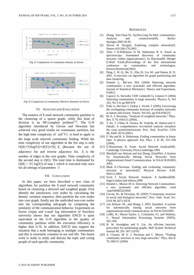
comparison of community density

0

10

20

30

1 2 3 4 5 6 7 8 9

communityID

D(communityID)

G-N

ENCD

Fig 11 Comparison of community density on Enron

comparision of community effective diameter

0

2

4

6

8

1 2 3 4 5 6 7 8 9

communityID

effective diameter

G-N

ENCD

Fig 12 Comparison of community effective diameter on Enron

VI. ANALYSIS AND EVALUATION

The essence of E-mail network community partition is the clustering of a sparse graph, while this kind of division is an NP-complete problem[12]. The G-N algorithm introduced by Girvan and Newman has achieved very good results on community partition, but the high time complexity of 2( )o E V is hard to apply to the large scale network community finding. While the time complexity of our algorithm in the fist step is only O(|E|+|V|log|V|)+O(|V|)+O(| cE |)because the use of adjacency list and inverse adjacency list. cE is the number of edges in the core graphs. Time complexity of the second step is O(E). The total time is dominated by O(|E| + |V| log|V|) of step 1 which is executed only once for all settings of parameters ∂ .

VII. CONCLUSION

In this paper, we have described a new class of algorithms for partition the E-mail network community based on clustering a directed and weighted graph. First identify the satisfactory core nodes by calculating the density variation sequence, then partition the core nodes into core graph, finally put the undivided non-core nodes into the corresponding sub-graph by computing the similarity of the communication behavior. Experiment on Enron corpus and e-mail log information of Soochow university shows that our algorithm ENCD is quite equivalent to the G-N algorithm in the quality of community partition while the execution efficiency is higher than G-N. In addition, ENCD also support the situation that a node belonging to multiple communities and this is extremely common in our real life. The future work is ready to study and discuss the topic and coring people of each specific community.

REFERENCES [1] Zhang Yan-Chun.Yu Xj,Hou.Ling-Yu.Web communities:

Analysis and construction[M]. Berlin: Springer,2005:56-92.

[2] Steven H. Strogatz. Exploring complex networks[J]. Nature,410:268-276,2001.

[3] Tyler J R,Wilkinson D M, Huberman B A. Email as spectroscopy: Automated discovery of community structure within organizations[c]. In HuysmanM, Wenger E,Wulf V.(eds.)Proceedings of the first international conference on communities and technologies, Kluwer,Dordrecht(2003)

[4] Ding, C. H. Q.; He, X.; Zha, H.; Gu, M.; and Simon, H. D. 2001. A min-max cut algorithm for graph partitioning and data clustering.

[5] Donetti L, Mu˜noz MA (2004) Detecting network communities: a new systematic and efficient algorithm. Journal of Statistical Mechanics: Theory and Experiment, P10012

[6] Capocci A, Servedio VDP, Caldarelli G, Colaiori F (2004) Detecting communities in large networks. Physica A, Vol 352, No 2-4, pp 669-676

[7] Palla G, Der'enyi I, Farkas I, Vicsek T (2005) Uncovering the overlapping community structure of complex networks in nature and society. Nature, Vol 435, pp 814-818[23]

[8] M. E. J. Newman, “Analysis of weighted networks.” Phys. Rev. E 70, 056131 (2004)..

[9] T. Ito, T. Chiba, R. Ozawa, M. Yoshida, M. Hattori,and Y. Sakaki, A comprehensive two-hybrid analysis toexplore the yeast proteininteractome. Proc. Natl. Acad.Sci. USA 98, 4569–4574 (2001).

[10] F. Wu and B. A. Huberman, Finding communities in linear time: A physics approach. Eur. Phys. J. B 38, 331–338 (2004).

[11] S.Wasserman, K. Faust. Social Network Analysis[M]. Cambridge University Press,Cambridge,1994

[12] Marshall van Alstyne and Jun Zhang. EmailNet: A System for Automatically Mining Social Networks from Organizational Email Communication. In NAACSOS2003, 2003.

[13] Mark E.J.Newman. Finding and evaluating community structure in networks[J]. Physical Review E,69. 026113,2004.

[14] Scott J. Social Network Analysis: A handbook[M]. Sage,London,2nd edition,2000

[15] Donetti L, Munoz M A. Detecting Network Communities: a new systematic and efficient algorithm. cond -mat/0404652(2004)

[16] Girvan, M., & Newman, M. (2002) “Community structure in social and biological networks”, Proc. Natl. Acad. Sci. USA 99, 8271-8276.

[17] van Alstyne, M., and Zhang, J. 2003. Emailnet: A system for automatically mining social networks from organizational email communication. In NAACSOS2003.

[18] Lodhi, H.; Shawe-Taylor, J.; Cristianini, N.; and Watkins, C. Neural Information Processing Systems (NIPS), 563–569

[19] B. W. Kernighan and S. Lin, An efficient heuristic proce-dure for partitioning graphs. Bell System Technical Journal 49, 291–307 (1970).

[20] A. Clauset, M. E. J. Newman and C. Moore, “Finding community structure in very large networks.” Phys. Rev.E 70, 066111 (2004)



Multiprocessor Scheduling by Simulated Evolution

Imtiaz Ahmad

Department of Computer Engineering Kuwait University, P. O. Box: 5969, Safat 13060 Kuwait


Muhammad K. Dhodhi Ross Video Ltd., 9 Slack Road, Ottawa, ON, K2G 0B7 Canada


Ishfaq Ahmad Department of Computer Science and Engineering

Box 19015, CSE, University of Texas at Arlington, Arlington, TX 76019 USA Email: [email protected]

Abstract— This paper presents a variant of simulated evolution technique for the static non-preemptive scheduling of parallel programs represented by directed acyclic graphs including inter-processor communication delays and contention onto a multiprocessor system with the dual objectives of reducing the total execution time and scaling with the number of processors. The premise of our algorithm is Simulated Evolution, an effective optimization method based on the analogy with the natural selection process of biological evolution. The proposed technique, named Scheduling with Simulated Evolution (SES), combines simulated evolution with list scheduling, wherein simulated evolution efficiently determines suitable priorities which lead to a good solution by applying list scheduling as a decoding heuristic. SES is an effective method that yields reduced length schedules while scaling well and incurring reasonably low complexity. The SES technique does not require problem-specific parameter tuning on test problems of different sizes and structures. Moreover, it strikes a balance between exploration of the search space and exploitation of good solutions found in an acceptable CPU time. We demonstrate the effectiveness of SES by comparing it against two existing static scheduling techniques for the test examples reported in literature and on a suite of randomly generated graphs. The proposed technique produced good quality solutions with a slight increase in the CPU time as compared with the competing techniques.

Index Terms— Software, Scheduling, Allocating Parallel Programs, Simulated Evolution

I. INTRODUCTION

Parallel programs are typically represented by directed acyclic graphs (DAGs). In a DAG, nodes denote tasks and an arc between any two nodes represents data dependency among them. The weights associated with the nodes and the arcs of a DAG represent the computation cost and the communication cost, respectively. The multiprocessor scheduling problem is

well known to be NP-complete except in a few restricted cases [1-2]. Hence, satisfactory suboptimal solutions obtainable in a reasonable amount of computation time are generally sought [3-13] by devising effective heuristics. The objective is not to propose another heuristic but to improve the effectiveness of a given heuristic.

Simulated evolution is a general purpose optimization method based on an analogy with the natural selection process in the biological environments. In biological processes, species adapt themselves to the environment as they evolve from one generation to the next. In this evolution process some of the bad characteristics of the old generation are eliminated and a new generation which is more suited to the environment is created [14-20]. Mutation and selection are the two main driving forces behind evolution. The simulated evolution models the evolution process by asexual reproduction with mutation and selection, while other probabilistic techniques, such as genetic algorithms [14], focus on recombination of different solutions via crossover and an occasional mutation. In the simulated evolution scheme mutation is the dominant operator and it is used for introducing variations into solutions. In nature, mutation refers to spontaneous and random changes in genes. The advantage is that optimization proceeds rapidly because the random distribution of new trials concentrates the computational effort on solutions that have provided evidence of success in the past [20]. Simulated evolution has been successfully applied to combinatorial optimization problems such as high-level synthesis [15], routing [16], circuit partitioning [17] and standard cell placement [18, 19]. A number of other evolutionary algorithms such as genetic algorithms [21], genetic list scheduling [22], particle swarm optimization [23], ant colony optimization [24] and artificial immune system [25] have been applied to multiprocessor scheduling problem with varying degree of success.



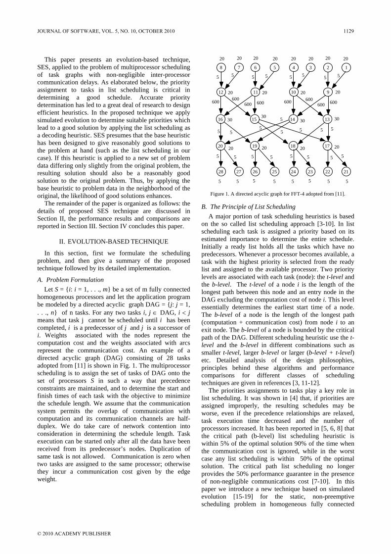
This paper presents an evolution-based technique, SES, applied to the problem of multiprocessor scheduling of task graphs with non-negligible inter-processor communication delays. As elaborated below, the priority assignment to tasks in list scheduling is critical in determining a good schedule. Accurate priority determination has led to a great deal of research to design efficient heuristics. In the proposed technique we apply simulated evolution to determine suitable priorities which lead to a good solution by applying the list scheduling as a decoding heuristic. SES presumes that the base heuristic has been designed to give reasonably good solutions to the problem at hand (such as the list scheduling in our case). If this heuristic is applied to a new set of problem data differing only slightly from the original problem, the resulting solution should also be a reasonably good solution to the original problem. Thus, by applying the base heuristic to problem data in the neighborhood of the original, the likelihood of good solutions enhances.

The remainder of the paper is organized as follows: the details of proposed SES technique are discussed in Section II, the performance results and comparisons are reported in Section III. Section IV concludes this paper.

II. EVOLUTION-BASED TECHNIQUE

In this section, first we formulate the scheduling problem, and then give a summary of the proposed technique followed by its detailed implementation.

A. Problem Formulation Let S = i: i = 1, . . ., m be a set of m fully connected

homogeneous processors and let the application program be modeled by a directed acyclic graph DAG = j: j = 1, . . ., n of n tasks. For any two tasks i, j ∈ DAG, i < j means that task j cannot be scheduled until i has been completed, i is a predecessor of j and j is a successor of i. Weights associated with the nodes represent the computation cost and the weights associated with arcs represent the communication cost. An example of a directed acyclic graph (DAG) consisting of 28 tasks adopted from [11] is shown in Fig. 1. The multiprocessor scheduling is to assign the set of tasks of DAG onto the set of processors S in such a way that precedence constraints are maintained, and to determine the start and finish times of each task with the objective to minimize the schedule length. We assume that the communication system permits the overlap of communication with computation and its communication channels are half-duplex. We do take care of network contention into consideration in determining the schedule length. Task execution can be started only after all the data have been received from its predecessor’s nodes. Duplication of same task is not allowed. Communication is zero when two tasks are assigned to the same processor; otherwise they incur a communication cost given by the edge weight.

8 1234567

28 21222324252627

20 171819

16 131415

12 91011

2020202020202020

20202020

303030

30

20202020

55555555

5 5 5 5 5 5 5 5

5 5 55

5

5 5 5

55555555

600 600600 600 600 600

600 600

Figure 1. A directed acyclic graph for FFT-4 adopted from [11].

B. The Principle of List Scheduling A major portion of task scheduling heuristics is based

on the so called list scheduling approach [3-10]. In list scheduling each task is assigned a priority based on its estimated importance to determine the entire schedule. Initially a ready list holds all the tasks which have no predecessors. Whenever a processor becomes available, a task with the highest priority is selected from the ready list and assigned to the available processor. Two priority levels are associated with each task (node): the t-level and the b-level. The t-level of a node i is the length of the longest path between this node and an entry node in the DAG excluding the computation cost of node i. This level essentially determines the earliest start time of a node. The b-level of a node is the length of the longest path (computation + communication cost) from node i to an exit node. The b-level of a node is bounded by the critical path of the DAG. Different scheduling heuristic use the t-level and the b-level in different combinations such as smaller t-level, larger b-level or larger (b-level + t-level) etc. Detailed analysis of the design philosophies, principles behind these algorithms and performance comparisons for different classes of scheduling techniques are given in references [3, 11-12].

The priorities assignments to tasks play a key role in list scheduling. It was shown in [4] that, if priorities are assigned improperly, the resulting schedules may be worse, even if the precedence relationships are relaxed, task execution time decreased and the number of processors increased. It has been reported in [5, 6, 8] that the critical path (b-level) list scheduling heuristic is within 5% of the optimal solution 90% of the time when the communication cost is ignored, while in the worst case any list scheduling is within 50% of the optimal solution. The critical path list scheduling no longer provides the 50% performance guarantee in the presence of non-negligible communications cost [7-10]. In this paper we introduce a new technique based on simulated evolution [15-19] for the static, non-preemptive scheduling problem in homogeneous fully connected



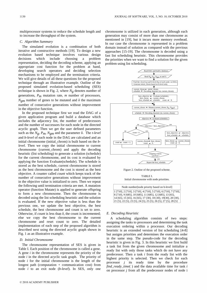
multiprocessor systems to reduce the schedule length and to increase the throughput of the system.

C. Algorithm Summary The simulated evolution is a combination of both

iterative and constructive methods [19]. To design a new evolution based technique involves various design decisions which include choosing a problem representation, deciding the decoding scheme, applying an appropriate cost function for the problem at hand, developing search operators and deciding selection mechanisms to be employed and the termination criteria. We will give details of all these questions for the proposed technique through an illustrative example. Outline of the proposed simulated evolution-based scheduling (SES) technique is shown in Fig. 2, where Ng denotes number of generations, Pm mutation rate, m number of processors, Ngm number of genes to be mutated and δ the maximum number of consecutive generations without improvement in the objective function.

In the proposed technique first we read the DAG of a given application program and build a database which includes the adjacency list, the number of predecessors and the number of successors for each node in the directed acyclic graph. Then we get the user defined parameters such as the Ng, Pm, Ngm and the parameter δ. The t-level and b-level of each node in the DAG are calculated and an initial chromosome (initial_chrom) is built based on the b-level. Then we copy the initial chromosome to current chromosome (current_chrom) and apply the decoding heuristic (list scheduling) to generate a solution (schedule) for the current chromosome, and its cost is evaluated by applying the function Evaluate(schedule). The schedule is stored as the best schedule, current chromosome is stored as the best chromosome and the cost is stored as the best objective. A counter called count which keeps track of the number of consecutive generations without improvement in the objective value is initialized to zero. Then we repeat the following until termination criteria are met. A mutation operator (function Mutate) is applied to generate offspring to form a new chromosome. Then the chromosome is decoded using the list scheduling heuristic and the solution is evaluated. If the new objective value is less than the previous one, we update the best objective, the best schedule, the best chromosome and count is set to zero. Otherwise, if count is less than δ, the count is incremented; else we copy the best chromosome to the current chromosome and reset count to zero. The detailed implementation of each step of the proposed algorithm is described next using the directed acyclic graph shown in Fig. 1 as an illustrative example.

D. Initial Chromosome The chromosome representation of SES is given in

Table I. Each position of the chromosome is called a gene. A gene i in the chromosome represents the priority of the node i in the directed acyclic task graph. The priority of node i for the initial chromosome is the length of the longest path (computation + communication cost) from node i to an exit node (b-level). In SES, only one

chromosome is utilized in each generation, although each generation may consist of more than one chromosome as mentioned in [19], but it incurs more memory overhead. In our case the chromosome is represented in a problem domain instead of solution as compared with the previous approaches [15-19]. The chromosome is decoded using a fast list scheduling heuristic. This chromosome provides the priorities when we want to find a solution for the given problem using list scheduling.

Read DAG and build a database;

yes

no

Read Ng, Pm, Ngm, m and δ

Find the t-level (ti) and b-level (bi) of each node i in DAG;Generate initial_chrom based on b-level only;

current_chrom initial_chrom;schedule Decoding_heuristic (m, current_chrom);

best_objective Evaluate (schedule);best_chrom current_chrom;

best_schedule schedule; count 0;

current_chrom Mutate (current_chrom, Pm, Ngm);

schedule Decoding_heuristic (m, current_chrom)

objective Evaluate (schedule);

objective < best_objectiveyesno

best_objective objective;best_schedule schedule;

best_chrom current_chrom; count 0;

no yescount > δ

current_chrom best_chrom; count 0; count count + 1;

Report the best_schedule.

stopping criteriasatisfied ?

;

Figure 2. Outline of the proposed scheme.

TABLE I.

Initial chromosome with node priorities.

Node number[node priority based on b-level] 1 [710], 2 [710], 3 [710], 4 [710], 5 [710], 6 [710], 7 [710], 8 [710], 9 [685], 10 [685], 11 [685], 12 [685], 13 [65], 14 [65], 15 [65], 16 [65], 17 [30], 18 [30], 19[30], 20 [30], 21 [5], 22 [5], 23 [5], 24 [5], 25 [5], 26 [5], 27 [5], 28 [5]

E. Decoding Heuristic A scheduling algorithm consists of two steps:

assigning the tasks to processors and determining the task execution ordering within a processor. Our decoding heuristic is an extended version of list scheduling [4-8] but assigns priorities and determines the execution order in the same step. The pseudo-code for the decoding heuristic is given in Fig. 3. In this heuristic we first build a task list from the given chromosome and initialize a ready list with only those tasks which do not have any predecessor. Then a task i from the ready list with the highest priority is selected. Then we check for each processor j its ready time by the procedure find_ready_time( ) and the data available time for task i on processor j from all the predecessor nodes of node i



the procedure find_data_available_time(i, j) by scheduling the messages on the links and taking into consideration the contention. The early start time for processor j is the maximum of its data available time and its ready time. We check this for all the processors and find a candidate processor on which task i can be started the earliest. Then the task i is scheduled onto candidate processor. Then the task i is deleted from the ready list. This process is repeated on the ready list till there is no task in the ready list. A task cannot be scheduled unless its predecessors have been scheduled and data has been communicated. The next_event gets the earliest time when a task finishes its execution. Then, at the next_event, tasks whose predecessors have been scheduled are inserted into the ready list at their appropriate position by a function called update_ready_list( ). If there is no ready task at the next_event, it is then assigned the earliest time at which at least one more running task completes its execution. The algorithm repeats these simple steps until the task list becomes empty.

Decoding_heuristic (chromosome, m): Build task_list from the chromosome; ready_list ← Initialize_ready_list(task_list); while (task_list < > null) do begin

for each task on the ready_list do begin Pick task i with the highest priority value; early_start_time = INFINITY; for j=1 to m begin pr_ready_time ← find_ready_time(j);

data_available_time ← find_data_available_time(i, j); pr_start_time=Max(data_available_time, pr_ready_time); If pr_start_time < early_start_time then begin candidate_processor = j; early_start_time = pr_start_time; end; end for;

Schedule task i onto candidate_processor; Delete task i from the ready_list;

end for; next_event ← find_time_for_ready_list_update( ); ready_list ← update_ready_list(next_event); end while; end Decoding_heuristic.

Figure 3. Pseudo-code of decoding heuristic.

For the illustrative example the tasks schedule on processors and links for the initial chromosome onto a multiprocessor system consisting of two homogeneous processors is shown in Table II. The schedule length is 2585 for the initial chromosome, which is more than serial time (480) because of the communication overhead. We store this solution and the corresponding chromosome in the database before introducing any variation in the chromosome.

F. Mutation In the simulated evolution based approach mutation is

the main operator which introduces variations in the chromosome to find new points in the search space. Usually mutation is implemented by selecting one gene at random, with a mutation rate Pm, and replacing its value. But our technique alters multiple numbers of genes given

by a parameter Ngm (the number of genes to be mutated) with a mutation rate Pm. The motivation behind mutating multiple genes at a time is to introduce enough variations into the chromosomes so that a different solution is generated by applying the decoding heuristic. If we mutate only one gene at a time, we need more generations to arrive at a good solution, hence requiring more CPU time. Pseudo-code for the mutation operator is shown in Fig. 4.

TABLE II. Initial schedule for Fig. 1.

Tasks scheduled on processors and links

P0

1 [0-20], 3 [20-40], 5 [40-60], 7 [60-80], 12 [85-105], 10 [105-125], 15 [1305-1335], 14 [1905-1935], 13 [2505-2535], 18 [2535-2555], 28 [2555-2560], 27 [2560-2565], 26 [2565-2570], 25 [2570-2575], 23 [2575-2580], 21 [2580-2585]

P1 2 [0-20], 4 [20-40], 6 [40-60], 8 [60-80], 11 [90-110], 9 [110-130], 16 [705-735], 20 [2510-2530], 19 [2530-2550],17 [2550-2570], 24 [2570-2575], 22 [2575-2580]

P0 xP1

(8 →12) [80-85], (5 → 11) [85-90], (4 → 10) [90-95], (1 → 9) [95-100], (12 → 16) [105-705], (11 → 15) [705-1305], (9 → 14) [1305-1905], (9 → 13) [1905-2505], (14 → 20) [2505-2510], (14 → 19) [2510-2515], (15 → 17) [2515-2520], (13 → 17) [2535-2540], (20 → 28) [2540-2545], (20 → 27) [2545-2550], (19 → 26) [2550-2555], (19 → 25) [2555-2560], (18 → 24) [2560-2565], (17 → 21) [2570-2575]

Note: 3 [20-40] means that node number 3 is scheduled on the processor from time units 20 to 40. (8 → 12) [80-85] means that a message from node 8 to node 12 is scheduled on the channel from time units 80 to 85 from the processor on which node 8 is assigned to the processor on which node 12 is assigned.

In the mutation operator, we randomly select Ngm number of genes with probability Pm and perturb their values in the range -t-levelj/2 to t-levelj/2, where t-levelj is the t-level of the node j in DAG with probability Pm . The priority of each node j in the chromosome is bounded in the range of b-levelj to b-levelj + t-levelj. If the priority value becomes more than b-levelj + t-level, the priority is assigned the value b-levelj + t-levelj. If the priority value becomes less than b-levelj, it is assigned the value b-levelj. The concept behind these ranges is to explore a wider space of priorities, but within the proximity to the original problem. After applying the mutation operator the old chromosome is replaced with a new one. The new generation is evaluated by applying the list scheduling heuristic. If the value of the objective function is less than the current best objective, the solution in the database is updated (i.e. the best objective is replaced with the new objective, best schedule gets new schedule).

G. Termination Criteria We always saved the chromosome which resulted in

the most recent best schedule. A counter count keeps track of the number of consecutive iteration without any improvement in the objective function value. When count becomes equal to δ, which is a user defined upper limit on the number of consecutive iterations without any improvement in the objective function value, we replace the current chromosome with the previous best chromosome and start the search again. This time we may go to a new neighborhood by altering the mutation rate or



also by increasing/decreasing the number of genes to be mutated. Since genes are picked up randomly, we will end up in a new neighborhood. This helps to escape from local optima, thereby enabling the search to continue. The best solution discovered by the proposed technique is stored separately and is updated when a new best solution is found during the search. We terminate the search when Ng generations are completed.

Mutation (chromosome, Pm, Ngm) for i= 1 to Ngm do begin j ← random (n, 1); r ← random ( ); if (r < Pm) then begin

chromosome[j] = chromosome[j] + random(- t-levelj/2, t-levelj/2); if (chromosome[j] > (t-levelj + b-levelj)) then

chromosome[j] = t-levelj + b-levelj; end if; if (chromosome[j] < b-levelj) then chromosome[j] = b-levelj; end if; end if;

end for; end Mutation.

Figure 4. Pseudo-code of mutation operator.

We experimented with various numbers of generations Ng, mutation rates Pm, the number of genes to be mutated (Ngm) which give good results at a reasonable computation cost. The number of generations between 50-150, Pm=0.6, and δ =10 are sufficient to arrive at reasonably good solutions. The effects of these parameters on schedule length are shown in the experimental results section. The final schedule and the chromosome which resulted in the best solution by applying the proposed technique to the DAG of Fig. 1 using two processors, is shown in Table III and Table IV, respectively. Note that the communication system allows overlap of communication with computation. SES generates a schedule length of 240, where both the processors are 100 % utilized. MH [9] and DLS [10] generate a schedule length of 2585 and 2635, respectively. One of the main drawbacks of MH is that it uses static priorities, while DLS does use dynamic priorities but the exploration space is very limited. The proposed technique outperforms all other techniques and provides the shortest schedule length. This example shows that priorities determination in list scheduling is the key element to determine a good schedule and the proposed scheme is providing a technique to exploit this feature.

TABLE III.

Chromosome which resulted in the best schedule for Fig. 1.

Node number[node priority] 1 [710], 2 [710], 3 [710], 4 [710], 5 [710], 6 [710], 7 [710], 8 [710], 9 [692], 10 [687], 11 [705], 12 [688], 13 [95], 14 [642], 15 [65], 16 [509], 17 [403], 18 [87], 19[541], 20 [476], 21 [418], 22 [16], 23 [19], 24 [58], 25 [220], 26 [147], 27 [706], 28 [384]

TABLE IV.

Schedule generated by SES for Fig. 1.

Tasks scheduled on processors and links

P0

1 [0-20], 3 [20-40], 5 [40-60], 7 [60-80], 11 [80-100], 12 [100-120], 16 [120-150], 15 [150-180], 19 [180-200], 17 [200-220], 27 [220-225], 21 [225-230], 26 [230-235], 23 [235-240]

P1 2 [0-20], 4 [20-40], 6 [40-60], 8 [60-80], 9 [80-100], 10 [100-120], 14 [120-150], 13 [150-180], 20 [180-200], 18 [200-220], 28 [220-225], 25 [225-230, 24 [230-235], 22 [235-240]

P0 xP1

(6 →11) [60-65], (1 → 9) [65-70], (8 → 12) [80-85], (3 → 10) [85-90], (14 → 19) [150-155], (16 → 20) [155-160], (13 → 17) [180-185], (15 → 18) [185-190], (20 → 27) [200-205], (19 → 25) [205-210], (18 → 23) [220-225], (17 → 22) [225-230]

III. EXPERIMENTAL RESULTS

The proposed simulated evolution-based technique, SES, for multiprocessor scheduling has been tested on a number of examples reported in literature and on a suite of randomly generated graphs. The results are very promising. The proposed evolution-based technique offers considerable improvement in the schedule length over previous work. We compared our results with the two competing techniques DLS [10] and MH [9]. For all the test examples the following values of different parameters were used: the number of generations (Ng) = 80; the mutation rate (Pm) =0.6; the number of genes to be mutated (Ngm) = 10; and the control parameter δ =10.

A. A Suite of Test Graphs [11] As a first example, we have selected a suite of test

graphs such as FFTs, trees (SUM1, SUM2) and irregular graph (IRR) used by McCreary et al. [11] to compare the performance of different scheduling algorithms. The FFT graph is shown in Fig. 1. The node weights for FFT-1 through FFT-3 are given in Table V. The communication cost is 25 units per edge for FFT-1 and FFT-2, while communication cost is 500 units per edge for FFT-3. The comparison of schedule lengths for all the test graphs is given in Table VI. The proposed technique gives the shortest schedule length as compared with the DLS and MH techniques for all the test cases.

TABLE V.

Nodes weight for FFTs graphs.

Node # FFT-1 FFT-2 FFT-3

1-8 1 60 20

9-12 20 50 20

13-16 30 5 30

17-20 20 5 20

21-28 1 5 5

B. Example 2 The second example consists of three different types of

directed acyclic graphs: Out-Tree, Fork-Join and Laplace Equation Solver. The comparison of schedule length with



DLS [10] and MH [9] techniques are given in Table VII. The proposed technique outperforms other techniques by providing a considerable improvement for all the test cases. This demonstrates the strength of the proposed technique to explore good solutions for different types of graph structures.

TABLE VI. Comparison of schedule lengths for test graphs of Example 1.

DAGs SES DLS [10] MH [9]

SUM-1 65 75 84

SUM-2 50 51 51

IRR 650 710 755

FFT-1 173 175 175

FFT-2 255 275 280

FFT-3 1630 2100 2570

The effects of different control parameters on the

schedule length for the Out-Tree graph are shown in Fig. 5. This Figure shows that if we mutate only one gene per generation like the traditional mutation operator, the solution quality does not improve with the number of generations (Ng) because the alterations in the chromosome are not enough to generate a different solution by applying the decoding heuristic. If we increase the value of Ngm the solution quality improves, because we are introducing enough variations into the chromosomes, so that a different solution is generated by applying the decoding heuristic. The solution quality depends mainly on the number of generations and on the value of Ngm. The mutation rate (Pm) does affect the solution quality, but impact appears only with an increase in the number of generations. With the increase in the number of generations, the solution quality certainly improves, but then it requires more CPU time. To achieve a reasonable balance between the quality of solution and the computation cost, one has to select suitable values of these parameters. The values of these parameters selected for our experimentation is a reasonable choice.

TABLE VII.

Comparison of schedule lengths for test graphs of Example 2.

DAGs SES DLS [10] MH [9]

Out-Tree 723 761 1070

Fork-Join 1924 3533 3406

Laplace 6390 7340 8370

C. A Suite of Random Graphs To demonstrate the effectiveness of our SES

technique, we consider a large suite of 175 of randomly generated graphs. The size of the graphs varied from 50 to 350 nodes with increments of 50. The cost of each node was randomly selected from a normal distribution with the mean equal to the specified average computation

cost. The cost of each edge was also randomly generated using a normal distribution with the mean equal to the product of the average computation cost and the communication-to-computation ratio (CCR). Five different values of CCR were selected: 0.1, 0.5, 1.0, 2.0, and 10.0. For generating the random task graphs, we used another parameter called parallelism (P). This parameter determines the average number of immediate descendents for each node. Five different values of parallelism were chosen: 1, 2, 3, 4, 5. Thus, the suite consists of 25 graphs for each size. We compared our results with the two competing techniques MH [9] and DLS [10] for 8 fully connected homogeneous processors. Two types of comparisons were carried out based on the results obtained by running each algorithm on this suite of 175 graphs. First, we compared the speedup for graphs with different values of CCR and P, and then we compared the average speedup for all the random graphs generated by the technique. Finally, we compared the average run times (CPU +I/O) of these algorithms. The discussion of these comparisons is as follows:

120100806040200600

700

800

900

1000

1100

1200

1300

1400 Pm=0.5, Ngm=1Pm=0.5, Ngm=4

Pm=0.75, Ngm=0.75Pm=0.5, Ngm=8

Number of generations

Sche

dule

leng

th

Figure 5. The effects of different parameters on the schedule length.

The typical pattern of speedup with different values of CCR is shown in Fig. 6-10. As the value of CCR is increased, the speedup decreases. The average speedup curves of SES, MH and DLS algorithms for 8 processors are given in Fig. 11. Each point in this figure is the average of 25 tests cases with various values of CCR and parallelism. We did not encounter a single instance during all the tests cases the schedule length generated by either DLS or MH are better than SES. The proposed technique outperformed both the MH and DLS algorithms. The average running times for various numbers of nodes in the task graph for 8 processors are given in Fig. 12. Each point in the figure is also the average of 25 tests cases. The running times of SES are large as compared with MH, but are comparable with DLS. The running times of SES becomes less as compared with DLS as the size of the graph is increased, since the overhead of the number of generations remains the same for all graph sizes. The proposed technique produces much better results in terms of the quality of the solution as compared with MH and DLS and with comparable running times with DLS.



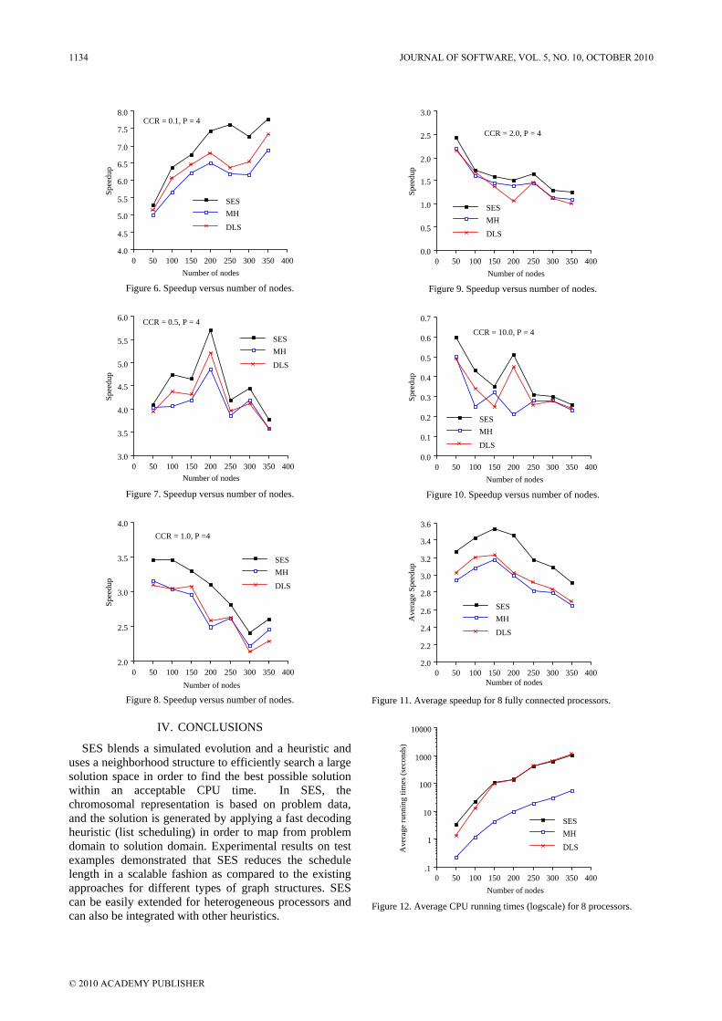
4003503002502001501005004.0

4.5

5.0

5.5

6.0

6.5

7.0

7.5

8.0

SESMH

DLS

CCR = 0.1, P = 4

Number of nodes

Spee

dup

Figure 6. Speedup versus number of nodes.

4003503002502001501005003.0

3.5

4.0

4.5

5.0

5.5

6.0

SESMH

DLS

CCR = 0.5, P = 4

Number of nodes

Spee

dup


4003503002502001501005002.0

2.5

3.0

3.5

4.0

SESMH

DLS

CCR = 1.0, P =4

Number of nodes

Spee

dup


IV. CONCLUSIONS

SES blends a simulated evolution and a heuristic and uses a neighborhood structure to efficiently search a large solution space in order to find the best possible solution within an acceptable CPU time. In SES, the chromosomal representation is based on problem data, and the solution is generated by applying a fast decoding heuristic (list scheduling) in order to map from problem domain to solution domain. Experimental results on test examples demonstrated that SES reduces the schedule length in a scalable fashion as compared to the existing approaches for different types of graph structures. SES can be easily extended for heterogeneous processors and can also be integrated with other heuristics.

4003503002502001501005000.0

0.5

1.0

1.5

2.0

2.5

3.0

SESMH

DLS

CCR = 2.0, P = 4

Number of nodes

Spee

dup


4003503002502001501005000.0

0.1

0.2

0.3

0.4

0.5

0.6

0.7

SESMH

DLS

CCR = 10.0, P = 4

Number of nodes

Spee

dup


4003503002502001501005002.0

2.2

2.4

2.6

2.8

3.0

3.2

3.4

3.6

SESMH

DLS

Number of nodes

Ave

rage

Spe

edup

Figure 11. Average speedup for 8 fully connected processors.

400350300250200150100500.1

1

10

100

1000

10000

SESMH

DLS

Number of nodes

Ave

rage

runn

ing

times

(sec

onds

)

Figure 12. Average CPU running times (logscale) for 8 processors.



REFERENCES

[1] M. R. Garey and D. S. Johnson, Computers and Intractability: A Guide to the Theory of NP Completeness, San Francisco, CA, W. H. Freeman, 1979.

[2] Y. Kwok and I. Ahmad, “Static Scheduling Algorithms for Allocating Directed Task Graphs to Multiprocessors,” ACM Computing Surveys, Vol. 31, No. 4, pp. 406-471, December 1999.

[3] Y. Kwok and I. Ahmad, “Benchmarking and Comparison of the Task Graph Scheduling Algorithms,” Journal of Parallel and Distributed Computing, Vol. 59, No. 2, pp. 381-422, December 1999.

[4] R. L. Graham, “Bounds on Multiprocessing Timing Anomalies,” SIAM Journal of Applied Math., 17, pp. 416-429, 1969.

[5] T. L. Adam, K. M. Chandy, and J. R. Dicson, “A Comparison of List Schedules for Parallel Processing Systems,” Communications of the ACM, Vol. 17, No. 12, pp. 685-690, December 1974.

[6] W. H. Kohler, “A Preliminary Evaluation of the Critical Path Method for Scheduling Tasks on Multiprocessor Systems,” IEEE Trans. on Computers, Vol. 24, No. 12, pp. 1235-1238, December 1975.

[7] C. Y. Lee, J. J. Hwang, Y. C. Chow, and F. D. Anger, “Multiprocessor Scheduling With Interprocessor Communication Delays,” Operations Research Letters, Vol. 7, No. 3, pp. 141-147, June 1988.

[8] T. Yang and A. Gerasoulis, “List Scheduling with and without Communication Delays,” Parallel Computing, 19, pp. 1321-1344, 1993.

[9] H. El-Rewini and T. G. Lewis, “Scheduling Parallel Program Tasks onto Arbitrary Target Machines,” Journal of Parallel and Distributed Computing, Vol. 9, No. 2, pp. 138-153, June 1990.

[10] G. C. Sih and E. A. Lee, “Scheduling to Account for Interprocessor Communication Within Interconnection-Constrained Processor Network,” 1990 International Conference on Parallel Processing, Vol. 1, pp. 9-17, August 1990.

[11] C. L. McCreary, A. A. Khan, J. J. Thompson, and M. E. McArdle, “A Comparison of Heuristics for Scheduling DAGs on Multiprocessors,” 8th International Parallel Processing Symposium, pp. 446-451, April 1994.

[12] G. Liao, E. R. Altman, V. K. Agarwal and G. R. Gao, “A Comparative Study of Multiprocessor List Scheduling Heuristics,” Twenty-Seventh Annual Hawaii International Conference on System Sciences, pp. 68-77, January 1994.

[13] Y Kwok and I. Ahmad, “Dynamic Critical-Path Scheduling: An Effective Technique for Allocating Task Graphs onto Multiprocessors,” IEEE Transactions on Parallel and Distributed Systems, Vol. 7, No. 5, pp. 506-521, May 1996.

[14] D. E. Goldberg, Genetic Algorithms in Search, Optimization and Machine Learning, Addison-Wesley, 1989.

[15] T. A. Ly and J. T. Mowchenko, “Applying Simulated Evolution to High Level Synthesis,” IEEE Trans. on CAD of Integrated Circuits and Systems, Vol. 12, No. 3, pp. 389-409, March 1993.

[16] Y. L. Lin, Y. C. Hsu, and F. S. Tsai, “SILK: A Simulated Evolution Router,” IEEE Trans. on CAD of Integrated Circuits and Systems, Vol. 8, No. 10, pp. 1108-1114, October 1989.

[17] Y. Saab and V. Rao, “An Evolution-Based Approach to Partitioning ASIC Systems,” 26th ACM/IEEE Design Automation Conference, pp. 767-770, 1989.

[18] Y. H. Hu and C. Y. Mao, “Solving Gate-Matrix Layout Problems by Simulated Evolution,” IEEE International Symposium on Circuits and Systems, pp. 1873-1875, 1993.

[19] R. M. King and P. Banerjee, “ESP: Placement by Simulated Evolution,” IEEE Trans. on CAD of Integrated Circuits and Systems, Vol. 8, No. 3, pp. 245-256, March 1989.

[20] V. Nissen, “Solving the Quadratic Assignment Problem with Clues from Nature,” IEEE Trans. on Neural Networks, Vol. 5, No. 1, pp. 66-72, January 1994.

[21] A. S. Wu, H. Yu, S. Jin, K. C. Lin and G. Schiavone, “An Incremental Genetic Algorithm to Multiprocessor Scheduling,” IEEE Trans. on Parallel and Distributed Computing, Vol. 15, No. 9, pp. 824-834, September 2004.

[22] M. Grajcar, “Genetic List Scheduling Algorithm for Scheduling and Allocation on a Loosely Coupled Heterogeneous Multiprocessor System,” Proceedings of the 36th Annual ACM/IEEE Design Automation Conference, pp. 280-285, 1999.

[23] T. Chen, B. Zhang, X. Hao and Y. Dai, “Task Scheduling in Grid based on Particle Swarm Optimization,” The Fifth international Symposium on Parallel and Distributed Computing, pp. 238-245, July 2006.

[24] C. Chiang, Y. Lee, C. Lee and T. Chou, “Ant Colony Optimization for Task Matching and Scheduling,” IEE-Proceedings Computers and Digital Techniques, Vol. 153, No. 6, pp. 373-380, November 2006.

[25] H. Yu, “Optimizing Task Schedules Using an Artificial Immune System Approach,” Proceedings of the 10th Annual Conference on Genetic and Evolutionary Computation, pp. 151-158, 2008.

Imtiaz Ahmad received his B.Sc. in Electrical Engineering from University of Engineering and Technology, Lahore, Pakistan, a M.Sc. in Electrical Engineering from King Fahd University of Petroleum and Minerals, Dhahran, Saudi Arabia, and a Ph.D. in Computer Engineering from Syracuse University, Syracuse, New York, in 1984, 1988 and 1992, respectively. Since September 1992, he has been with the Department of Computer Engineering at Kuwait University, Kuwait, where he is currently a professor. His research interests include design automation of digital systems, high-level synthesis, and parallel and distributed computing.

Muhammad K. Dhodhi received his B.Sc. (with honors) in Electrical Engineering from the University of Engineering and Technology, Lahore, Pakistan in 1982. He received two Master degrees, one in Computer and Systems Engineering and another in Electric Power Engineering, from Rensselaer Polytechnic Institute, Troy, New York, in 1984 and 1986, respectively. He received a Ph.D. in Electrical Engineering from Lehigh University, Bethlehem, PA, in 1992. Dr. Dhodhi has research and development experience both in the industry as well as in academia. Dr. Dhodhi is currently a Senior Member of hardware development team at Ross Video Ltd., Ottawa, Canada. In the past, he has worked as a member of technical staff for distinguished global organizations such as Nortel Networks, Lucent Technologies, IBM Corporation, and a number of start-ups such as Diablo Technologies, Silicon Optix, The VHDL Technology Group, Silc Technologies and as a Principal Consultant at Hayat ECAT, Inc. In industry, Dr. Dhodhi has been actively involved in all the phases of VLSI design, modeling and verification of System-on-Chip (SoC)



devices, ASICs/FPGAs used in Networking (i.e., Multiservice Core Switching Products, Terabit Switch Routers), Video/Image Processors, and Advanced Memory Buffers for DDR2/DDR3. He has also played a key role in the development of state-of-the-art constrained random versification and assertion-based design and verification methodologies.

In academia, Dr. Dhodhi had worked as an assistant professor with the Department of Electrical and Computer Engineering, Kuwait University, from February 1993 to May 1997. He was an associate professor of electrical and computer engineering, Kuwait University, Kuwait from 1997 to 1998. Dr. Dhodhi research interests are in Wireless Sensor Networks, Hardware/Software Co-Design Verification, VLSI Design Automation and Parallel/Distributed Computing.

Ishfaq Ahmad received a B.Sc. degree in Electrical

Engineering from the University of Engineering and Technology, Pakistan, in 1985, and an MS degree in Computer Engineering and a PhD degree in Computer Science from Syracuse University, New York, U.S.A., in 1987 and 1992, respectively. He is currently a professor of Computer Science and Engineering at the University of Texas at Arlington (UTA). Prior to joining UTA, he was on the faculty of Computer Science Department at the Hong Kong University of Science

and Technology (HKUST). At UTA, he leads the Multimedia Laboratory and the Institute for Research in Security (IRIS). IRIS, an inter-disciplinary research center spanning several departments, is engaged in research on advanced technologies for homeland security and law enforcement. Professor Ahmad is known for his research contributions in parallel and distributed computing, multimedia computing, video compression, and security. His work in these areas is published in 200 plus technical papers in peer-reviewed journals and conferences.

Dr. Ahmad is a recipient of numerous research awards, which include three best paper awards at leading conferences and 2007 best paper award for IEEE Transactions on Circuits and Systems for Video Technology, IEEE Service Appreciation Award, and 2008 Outstanding Area Editor Award from the IEEE Transactions on Circuits and Systems for Video Technology.

His current research is funded by the Department of Justice, National Science Foundation, SRC, Department of Education, and several companies. He is an associate editor of the Journal of Parallel and Distributed Computing, IEEE Transactions on Circuits and Systems for Video Technology, IEEE Transactions on Multimedia, IEEE Distributed Systems Online, and Hindawi Journal of Electrical and Computer Engineering. He is a Fellow of the IEEE and a member of the advisory board of Lifeboat Foundation.



The Chinese Text Categorization System with Category Priorities

Huan-Chao Keh

Department of Information Engineering, Tamkang University, Taipei, Taiwan Email: [email protected]

Ding-An Chiang, Chih-Cheng Hsu and Hui-Hua Huang

Department of Information Engineering, Tamkang University, Taipei, Taiwan Email: [email protected], [email protected], [email protected]

Abstract—The process of text categorization involves some understanding of the content of the documents and/or some previous knowledge of the categories. For the content of the documents, we use a filtering measure for feature selection in our Chinese text categorization system. We modify the formula of Term Frequency-Inverse Document Frequency (TF-IDF) to strengthen important keywords’ weights and weaken unimportant keywords’ weights. For the knowledge of the categories, we use category priority to represent the relationship between two different categories. Consequently, the experimental results show that our method can effectively not only decrease noise text but also increase the accuracy rate and recall rate of text categorization. Index Terms—text categorization, feature selection, filtering measure, text mining

I. INTRODUCTION

English is taken as the main language family in many recent text mining studies [1][2][3]. Chinese language family studies are not common. Therefore, we have a fact study of Chinese text categorization system. In Chinese text, there are no obvious spaces between Chinese words and English words, numbers, and symbols are often included, so the feature extraction needs punctuation. Chinese punctuation is to divide particular text into some words of uncertain lengths. Since a single Chinese character has different meanings when combined with different characters, Chinese punctuation has to rely on a large word library and context comparison in order to acquire the most appropriate words. As this system only categorizes Chinese articles, in the preprocess phase, we remove all characters except Chinese words and use the Chinese Punctuation System [4], developed by Library Team of Central Research Academy, to make Chinese punctuation. We find that some features may be missed or divided into different features with different meanings; for example “大腸桿菌” (colon bacillus) is cut into “大腸”(colon) and “桿菌” (bacillus), though “大腸桿菌”(colon bacillus) should be regarded as a single feature. Although some features may not be cut out from one feature, the correlation between these features exists. If this type of combining feature is regarded as a special feature, it will be helpful in

classification processing. The association rule can be used to find terms which may have relations to each other. Therefore, we utilize the associative classification technique to deal with such subject in ref. [5].

In this paper, we use feature terms longer than two characters to compute weights of these terms relative to categories. After being punctuated, the document can be represented by the bag of words [1]. The document D can be converted to d= ((f1,w1),(f2,w2)…(fi,wi)), where each fi is a document word, and wi denotes its frequency. Since the number of different words appearing in the collection may be very large and contain many irrelevant words for the classification, in addition to eliminating stop words and auxiliary words such as「的

」(of),「而且」(but also),「和」(and),「因爲」(because), feature reduction is usually performed. As pointed out by ref. [3], filtering and wrapping are two main approaches to feature reduction. Since wrapper approaches are time-consuming and sometimes unfeasible to use, in this paper, we use filtering measure, TF-IDF, for feature selection in our text categorization system. Although the TF-IDF is performed well in many situations [6], this formula still has some problems. To solve these problems, we will modify this formula to improve the classification recall rate and accuracy rate. We introduce this improved formula in section 3.

The data sources of this study are from the thesis abstracts of universities in Taiwan. These thesis abstracts are extracted from “National Dissertations and Theses Information Web” [7]. Generally, documents are classified into different categories by the content of the document directly. However, documents are thesis abstracts in this research and some theses of a department may cross different fields. If we do not consider previous knowledge of the categories, theses should be categorized by departments which release the theses, and only consider the content of these theses, it may cause classification errors. For example, some theses of the chemistry department may apply related chemistry knowledge to the field of biology, thus in document classification, it may be wrongly classified into the “Biology” category because of many biological keywords in these abstracts. In this paper, we use category priority to solve this kind of classification



mistake. The category priority will be introduced in section 3.

The rest of this paper is organized as follows: In Section 2, related work is summarized. In Section 3, improved TF-IDF method and category priorities are presented. Section 4 introduces experiment results. In section 5, conclusions and further research are described.

II. RELATIVE WORK

A. Document Classification Process The different text categorization systems have been

proposed recently [8][9][10][11], in this paper, we refer Aas and Eikvil [12] and sum up the systemic process for document classification as shown in Fig. 2.1. The system classified documents as training documents and test documents, pretreated training documents with known categories and extracted all kinds of feature terms through phrase distribution statistics, retained meaningful phrases and built the classification estimation model, then categorized the test documents.

Before document classification, we have to select and determine a document profile. Titles, abstracts or specified chapters can be taken as document profiles. If all document content is selected as the document profile, there would be a huge amount of text information and a lot of meaningless information. The document profile shall therefore be selected according to category feature and shall be the most representative content. The proper document profile can reduce redundant text information so as to enhance classification performance. For example, Maron [10] took Transaction on Electronic Computer periodicals as a document source, and

selected abstracts as document profiles. Hamill [8] took Chemical Abstracts Titles as document profiles.

Feature extraction is further divided into pre-process, document representation and feature selection. In this part, most of the related literature are English documents as test data source. If Chinese documents are to be tested; in the feature extraction part, a Chinese punctuation treatment must be additionally done. After being punctuated, in addition to eliminating stop words and auxiliary words, we have to perform feature selection to reduce the affect of irrelevant words on classification.

B. Weight Computation Feature extracted documents are often expressed as

vector patterns (weight, keyword). The weight can be computed by different methods, such as information gain [10][13], mutual information [10], etc. As pointed out by ref. [14], the TF-IDF method performs well in many situations. In this paper, we use this filtering measure method in our system and it is introduced as follows.

The TF-IDF method uses the term frequency and document frequency to compute the weight of a word in a document. The term frequency TF(t,d) is the frequency of a word t in the document d. The document frequency DF(t) is the number of documents that contain a word t. The inverse document frequency of a word t, IDF(t), can be computed by the following formula:

(1)

In the above formula, D is the number of documents

and IDF(t) is the discretion degree of a word t over the integral document. Since the importance of a word t in a document d is proportional to the frequency of a word occurring in a document and inverse document frequency, the weight of a word t in a document d, W(t,d), can be computed by the following formula:

W(t,d) = TF(t,d)× IDF(t) (2)

In the above formula, a larger value of W(t,d) indicates a higher frequency of a word t occurring in a document d, but a lower frequency of t occurring in all documents.

The problem with this formula is that it easily results in constant IDF(t) of term t at each category, or very similar weights of term t with respect to various categories. When this situation occurs, the weight of t in different document d totally depends on the term frequency TF(t,d). When the frequency of a noise term, TF(t,d), is higher, the weight W(t,d) with respect to each category will be bigger; therefore, the classification error probability will increase. To improve the classification accuracy, the discretion should take account of category distribution of each word. This article primarily adopted TF-IDF weight method and made some improvements. The modified TF-IDF will be introduced in the next section.

⎥⎦

⎤⎢⎣

⎡=

)(log)(

tDFDtIDF

Document Classification Process

Training Document

Feature ExtractionPre-Process

Document Representation

Feature Selection

Class A Class B Class C

Classifier

Test Document Class Keywords

Database

Figure 2.1 The process of text categorization system



C. Classification Many document classification algorithms, such as

Rocchio classification [15][16], decision tree classification [17], SVM(support vector machine)[18], KNN nearest neighbor rule [19], and Naïve-Bayes [13][20], have seen proposed recently. Various classification algorithms have their own advantages and different classification models. In this paper, we use Naïve-Bayes classification method to classify documents; therefore, only this method is introduced in this section.

Naïve-Bayes classification method is designed on the basis of Bayesian analysis theory. Bayesian Analysis was proposed by Thomas Bayes in the early 18th century. Its basic principle is to modify (or improve) boundary probability of a certain incident according to some additional information. It predicts the probability of an object being the member of a certain category so as to complete classification. This study adopted Bayes probability [13][20] as the classification criterion. For the Naïve-Bayes classifier, this paper calculates the weights of all characteristic terms according to TF-IDF formula. For test documents, Bayes performs as the basis of the classification rules. It makes the occurrence number of characteristic terms<f1,f2,f3…,fi> of a document(j) and multiplies its matched IDF. The obtained weight is the cumulative integral of that class provided that the number of the classes is known. And then it sums the cumulative integral of one class in the document to get the matched integral for that class. Based on the obtained matched integral, it can infer the class of this document through the following formula:

∑ ×= )|()()( jiwfitermjValue (3)

where Value(j) is the cumulative integral of each document. Based on this probability data, we classify this uncategorized data to the category with highest the probability.

III. SYSTEM

A. Process of the system As shown in figure 3.1, the proposed system firstly

summarizes the occurrence of each term in training documents and uses improved TF-IDF to build weighting table. Thereby, the system computes the sum of the weight of each test document relative to each category. In addition, as the document has cross-field property, the highest weight or second highest weight will be selected as the final classification result, on the basis of category priority.

B. TF-IDF Improvement The traditional TF-IDF method did not consider the

distribution of feature terms over different categories; therefore, it may not only discriminate important words since they occur less times in the document, but may also be less useful in reducing noise terms because IDF(t) is close to zero. To differentiate meaningless noise terms and important feature terms, the category

distribution of feature terms should be taken into consideration. Accordingly, the improved TF-IDF formulas are given as bellows:

W(t,c)=TF(t,c) × IDF(t,c) (4)

2

βαlog

DF(t)Dlog

,c)TF(t)-TF(tTF(t)logIDF(t) ⎥

⎦

⎤⎢⎣

⎡×⎥⎦

⎤⎢⎣

⎡×⎥⎦

⎤⎢⎣

⎡+

=1

　 (5)

where，TF(t)：frequency of term t TF(t,c)：frequency of term t at category c D：total number of documents DF(t)：document frequency of term t α：total number of categories β：number of category where term t appears

The improved IDF is composed of three items: the first item is to determine discretion of term t by its concentration at one category, that is, the higher the occurrence of term t is at the category, the smaller the denominator is (near 1). The lower the occurrence of term t at the category, the bigger the denominator (near numerator) so that IDF gets lower; the second item is traditional IDF; the third item is to determine the distribution of term t over categories by quantity of categories where term t is distributed. If term t appears at only a few categories, then IDF will rise; however, if term t appears at multiple categories, then IDF will fall.

For example, as shown in Table 3.1, the traditional TF-IDF weighting method fails to filter the unimportant words “研究” (study) and “結果”(result). Unlike the traditional TF-IDF weighting method, the improved TF-IDF method is able to use category distribution parameter to reduce the influence of noise terms. As shown in Table 3.1, weights of “研究” (study) and “結果”(result) are reduced to zero.

Figure 3.1 Process of the system



TABLE 3.1 AFTER IMPROVED, THE WEIGHT OF USELESS KEYWORD IS WEAKENED

Class Feature Class Freq.

Total Freq.

Class Num.

Traditional TF-IDF

Improved TF-IDF

大氣 Atmosphere

研究 Study

298 5394 6 34.65 0.0

大氣 Atmosphere

結果 Result

370 2199 6 90.25 0.0

音樂 Music

研究 Study

492 5394 6 57.21 0.0

音樂 Music

結果 Result

68 2199 6 16.59 0.0

化學 Chemistry

研究 Study

455 5394 6 52.91 0.0

化學 Chemistry

結果 Result

332 2199 6 80.98 0.0

教育 Education

研究 Study

2446 5394 6 284.43 0.0

教育 Education

結果 Result

344 2199 6 83.91 0.0

土木 Civil

研究 Study

1309 5394 6 152.22 0.0

土木 Civil

結果 Result

728 2199 6 177.57 0.0

生物 Biology

研究 Study

394 5394 6 45.82 0.0

生物 Biology

結果 Result

357 2199 6 87.08 0.0

Another example shows that, according to distribution

at various categories, the improved TF-IDF method can strengthen or weaken the importance of the same keyword with respect to different categories at the same time. For example, as shown in table 3.2, “颱風” (typhoon) has weight at both “Civil” category and “Atmosphere” category. Comparing with the weights of “颱風” (typhoon) of the improved TF-IDF and that of the traditional TF-IDF weighting method, obviously, the weight of “颱風” (typhoon) at category “Civil” is weakened; and another example, “鋼琴” (piano) has weight at both “Music” and “ Education” categories. After being improved, the weight at category “Music” was strengthened and at “ Education” is reduced to zero. Therefore, the improved TF-IDF method can strengthen keyword differentiation at various categories, so as to increase classification accuracy.

C. Category Priority As mentioned in the introduction, the data sources are

thesis abstracts of universities in Taiwan and are classified by departments which release the theses in this study. Since some theses may cross two different departments, this situation may cause classification error. For example, a document originally belonging in the “Chemistry” category with an abstract that contains biological keywords, such as “bacteria”, “infection”, etc, will be classified in the “Biology” category because the weight relative to “Biology” is greater than to “Chemistry”. In order to identify the major department

TABLE 3.2 AFTER IMPROVED, VARIATION OF KEYWORD AT DIFFERENT

CATEGORIES ARE STRENGTHENED

Class Feature Class Freq.

Total Freq.

Class Num.

Traditional TF-IDF

Improved TF-IDF

音樂 Music

作品 Work

518 539 2 618.66 820.09

教育Education

作品 Work

21 539 2 25.08 0.39

教育Education

音樂Music

45 1162 2 46.56 0.74

音樂 Music 音樂Music

1117 1162 2 1155.67 1546.59

大氣Atmosphere

氣流 Air flow

199 201 2 290.97 507.03

土木 Civil 氣流 Air flow

2 201 2 2.92 6.04

土木 Civil 混凝土Concrete

582 587 2 718.18 1364.12

化學Chemistry

混凝土Concrete

5 587 2 6.17 1.75

生物 Biology

蛋白Protein

997 1018 2 1053.47 1674.09

化學Chemistry

蛋白Protein

21 1018 2 22.19 0.18

土木 Civil

颱風Typhoon

33 368 2 52.95 1.99

大氣Atmosphere

颱風Typhoon

335 368 2 537.50 530.54

音樂 Music

鋼琴 Piano

317 318 2 485.41 1019.68

教育Education

鋼琴 Piano

1 318 2 1.53 0.0

of these theses, different priorities should be given to these two different categories. In this paper, we propose a simple approach, category priority, to solve this problem. Since we found that, the chemistry department often produces theses similar to biology, but the biology department seldom produces theses similar to chemistry, we can use category priority to describe the above relationship of this kind of cross-field theses. In this case, the priority of the “Chemistry” category is higher than that of the “Biology” category and this relationship can be represented as follow:

Chemistry Biology. (6)

Moreover, since these theses are crossing biology and chemistry fields, weights of these theses relative to the “Chemistry” category and the “Biology” category should be higher than those to other departments. Accordingly, we can define the following algorithm, as shown in the following algorithm, to classify cross-field theses.

The Algorithm Classify Cross-Field Theses.

/* Let the document D be a thesis crossing “A” and “B” fields, and the category priority of “A” be higher than that of “B”*/



If the weight of thesis to “A” is highest, Then this thesis belongs to “A” category, Else if the ratio of weight between “A” and “B” reaches a certain threshold, Then this thesis belongs to “A” category, Else this thesis belongs to “B” category. To classify these theses which are crossing biology

and chemistry fields by the above algorithm, we can select the documents where the highest weight is the “Biology” category and second highest weight is the “Chemistry” category. If the ratio of weight between the “Chemistry” category and the “Biology” category reaches a certain threshold, we can classify this document to the “Chemistry” category according to its second highest weight. This study sets the threshold as 0.6 by the experimental experience. For example, comparing the experimental results of using the improved TF-IDF method without and with category priorities, as shown in Table 3.3, when category priority Chemistry Biology is used, there are 15 theses are classified from “Biology” category into “Chemistry” category and 14 theses are classified correctly.

TABLE 3.3 NUMBER OF DOCUMENTS ARE CLASSIFIED FROM ORIGINAL CATEGORY

TO NEW CATEGORY BY THE IMPROVED TF-IDF WITH CATEGORY PRIORITIES

Highest Class

Second Class

Effected Doc.

Wrong Correct

CorrectWrong

WrongWrong

生物 Biology

化學 Chemistry

15 14 1 0

土木 Civil

化學 Chemistry

10 8 1 1

教育 Education

土木 Civil

13 9 2 2

Moreover, some theses of the chemistry department may also apply related chemistry knowledge to the field of the civil department, thus in document classification, it may be wrongly classified into the “Civil” category. For example, a document originally belonging in the “Chemistry” category which has an abstract that contains keywords of a “Civil engineering” nature, such as “concrete”, “cement”, etc, will be classified in the “Civil” category because the weight relative to “Civil” is greater than to “Chemistry”. For the same reason between the “Chemistry” category and the “Biology” category, we define that the priority of the “Chemistry” category is higher than that of the “Civil” category. This relationship can be represented as follow:

Chemistry Civil. (7)

As shown in Table 3.4, when the traditional TF-IDF method and category priority Chemistry Civil are used, there are 65 theses which are classified from the “Civil” category into the “Chemistry” category and 52 theses are correctly classified. Moreover, as shown in Table 3.3, when improved TF-IDF method and category priority Chemistry Civil are used, there are 10 theses classified from the “Civil” category into the “Chemistry” category and 8 theses are classified

correctly. Clearly, the accuracy rate and recall rate are improved when category priorities are used.

TABLE 3.4 NUMBER OF DOCUMENTS ARE CLASSIFIED FROM ORIGINAL CATEGORY

TO NEW CATEGORY BY THE TRADITIONAL TF-IDF WITH CATEGORY PRIORITIES

Highest Class

Second Class

Effected Doc.

Wrong Correct

CorrectWrong

WrongWrong

生物 Biology

化學 Chemistry

31 15 15 1

土木 Civil

化學 Chemistry

65 52 8 5

教育 Education

土木 Civil

26 16 4 6

IV. EXPERIMENTAL RESULTS

This article selected 6065 thesis abstracts from the “National Dissertations and Theses Information Web” as the document profile, and categorized them on the basis of six departments [7]. The thesis distribution is shown in Table 4.1. We select 10% of the documents as training data to build a classification model, and 30% of the documents as testing data.

TABLE 4.1 NUMBER OF DOCUMENTS SELECTED FROM EACH DEPARTMENT

Dept. Name Document Num. 土木 Civil 1794

生物 Biology 1004

化學 Chemistry 1003

大氣 Atmosphere 670

音樂 Music 658

教育 Education 936

Total 6065 After analysis, it was found that Chinese and English

words are mixed in thesis abstracts, documents of the chemistry department contain abbreviated chemistry formulae and compound names, and a minority of articles has no abstracts. Therefore, we have to remove characters except Chinese words and use the Chinese Punctuation System [4] to make Chinese punctuation. Moreover, since theses may cross two different fields, we have to define the category priorities before classification. The category priorities with respect to these six departments are:

Chemistry Biology. (8) Chemistry Civil. (9)

Civil Education. (10)

After that, we use traditional TF-IDF method and improved TF-IDF method with and without category priority to classify documents. The effect of document classification can be evaluated by Recall rate and Accuracy rate, while Recall rate and Accuracy rate for a category “A” are defined as follows:

Recall rate = α / (β+α) (11)

Accuracy rate= α / (γ+α) (12)



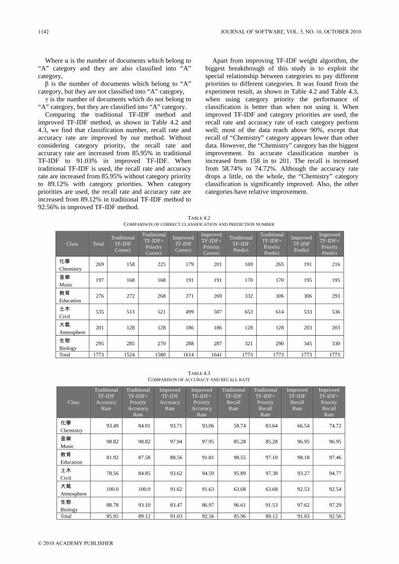
Where α is the number of documents which belong to “A” category and they are also classified into “A” category, β is the number of documents which belong to “A”

category, but they are not classified into “A” category, γ is the number of documents which do not belong to

“A” category, but they are classified into “A” category. Comparing the traditional TF-IDF method and

improved TF-IDF method, as shown in Table 4.2 and 4.3, we find that classification number, recall rate and accuracy rate are improved by our method. Without considering category priority, the recall rate and accuracy rate are increased from 85.95% in traditional TF-IDF to 91.03% in improved TF-IDF. When traditional TF-IDF is used, the recall rate and accuracy rate are increased from 85.95% without category priority to 89.12% with category priorities. When category priorities are used, the recall rate and accuracy rate are increased from 89.12% in traditional TF-IDF method to 92.56% in improved TF-IDF method.

Apart from improving TF-IDF weight algorithm, the biggest breakthrough of this study is to exploit the special relationship between categories to pay different priorities to different categories. It was found from the experiment result, as shown in Table 4.2 and Table 4.3, when using category priority the performance of classification is better than when not using it. When improved TF-IDF and category priorities are used, the recall rate and accuracy rate of each category perform well; most of the data reach above 90%, except that recall of “Chemistry” category appears lower than other data. However, the “Chemistry” category has the biggest improvement. Its accurate classification number is increased from 158 in to 201. The recall is increased from 58.74% to 74.72%. Although the accuracy rate drops a little, on the whole, the “Chemistry” category classification is significantly improved. Also, the other categories have relative improvement.

TABLE 4.2 COMPARISON OF CORRECT CLASSIFICATION AND PREDICTION NUMBER

Class Total Traditional

TF-IDF Correct

Traditional TF-IDF+ Priority Correct

ImprovedTF-IDF Correct

ImprovedTF-IDF+Priority Correct

TraditionalTF-IDF Predict

Traditional TF-IDF+ Priority Predict

Improved TF-IDF Predict

ImprovedTF-IDF+Priority Predict

化學 Chemistry

269 158 225 179 201 169 265 191 216

音樂 Music

197 168 168 191 191 170 170 195 195

教育 Education

276 272 268 271 269 332 306 306 293

土木 Civil

535 513 521 499 507 653 614 533 536

大氣 Atmosphere

201 128 128 186 186 128 128 203 203

生物 Biology

295 285 270 288 287 321 290 345 330

Total 1773 1524 1580 1614 1641 1773 1773 1773 1773

TABLE 4.3 COMPARISON OF ACCURACY AND RECALL RATE

Class

Traditional TF-IDF

Accuracy Rate

Traditional TF-IDF+ Priority

Accuracy Rate

Improved TF-IDF

Accuracy Rate

Improved TF-IDF+ Priority

Accuracy Rate

Traditional TF-IDF Recall Rate

Traditional TF-IDF+ Priority Recall Rate

Improved TF-IDF Recall Rate

Improved TF-IDF+ Priority Recall Rate

化學 Chemistry

93.49 84.91 93.71 93.06 58.74 83.64 66.54 74.72

音樂 Music

98.82 98.82 97.94 97.95 85.28 85.28 96.95 96.95

教育 Education

81.92 87.58 88.56 91.81 98.55 97.10 98.18 97.46

土木 Civil

78.56 84.85 93.62 94.59 95.89 97.38 93.27 94.77

大氣 Atmosphere

100.0 100.0 91.62 91.63 63.68 63.68 92.53 92.54

生物 Biology

88.78 93.10 83.47 86.97 96.61 91.53 97.62 97.29

Total 85.95 89.12 91.03 92.56 85.96 89.12 91.03 92.56



V. CONCLUSION

In this paper, we improve traditional TF-IDF to compute terms’ weights. Besides, in order to cope with interdisciplinary research case, we introduce category priorities to solve cross fields problem. It does not select the highest weighted category, but chooses the second highest weighted category in some cases. The experiment results verified that it can get better classification results than when not using category priority.

This study is to categorize Chinese documents, and the results may also be achieved when applying it to process English documents. We also plan to use weighted classification method coupled with data mining approach to find some useful rules so as to increase classification accuracy. These shall serve as the direction of our further study.

REFERENCES

[1] V. Vapnik , S. Golowich, and A. Smola, “Support vector method for function approximation, regression estimation, and signal Processing,” Neural Information Processing Systems 9, pp. 281-287, 1997

[2] Y. Huang, J. Tan, and L. Zhang, “A context analytical method basing on text structure,” Journal of Software, vol. 4, no. 1, pp.3-10, February 2009.

[3] J. Myung, J.-Y. Yang, and S.-G. Lee, ”Picachoo: A text analysis tool for customizable feature selection with dynamic composition of primitive methods,” Journal of Software, vol. 5, no. 2, pp.179-186, February 2010.

[4] Language and Knowledge Processing Group, Institute of Information Science, Academia Sinica, “Chinese Word Segmentation System,” http://ckipsvr.iis.sinica.edu.tw/.

[5] D. A. Chiang, H. C. Keh, H. H. Huang, and D. Chyr, ”The chinese text categorization system with association rule and category priority,” Expert Systems with Applications, vol. 35, no. 1-2, pp. 102-110, 2008.

[6] I. Díaz, J. Ranilla, N. Elena Monta, J. Fernández, and E. F. Combarro, ”Improving performance of text categorization by combining filtering and support vector machines: Research articles,” J. Am. Soc. Information Science and Technology, vol. 55, no. 7, pp. 579-592, May 2004.

[7] National Central Library, “Electronic Theses and Dissertations System,” http://etds.ncl.edu.tw/theabs/index.jsp.

[8] K. A. Hamill and A. Zamora, ”The use of titles for automatic document classification,” Journal of the

American Society for Information Science, vol. 31, no. 6, pp. 396-402, 1980.

[9] K. L. Kwok, “The Use of Title and Cited Titles as Document Representation for Automatic Classification,” Journal of Information and Management, Vol. 11, pp. 201-206, 1975.

[10] M.E. Maron, “Automatic Indexing : an Experimental Inquiry,” J. of the ACM, Vol. 8, pp. 404-417, 1961.

[11] Tom M. Mitchell, “Machine Learning,” The McGraw-Hill Companies, Inc, 1997.

[12] K. Aas and L. Eikvil. “Text categorisation: A survey,” Technical report, Norwegian Computing Center, 1999.

[13] Mingyu Lu, Keyun Hu, Yi Wu, Yuchang Lu, and Lizhu Zho, “SECTCS: towards improving VSM and Naive Bayesian classifier:Systems, Man and Cybernetics,” IEEE International Conference on 2002 , Vol. 5, pp. 6-9, Oct. 2002.

[14] Elı´as F. Combarro, Elena Montan˜e´ s, Irene Dı´az, Jose´ Ranilla, and Ricardo Mones, “Introducing a Family of Linear Measures for Feature Selection in Text Categorization,” IEEE Transactions on knowledge and data engineering, vol. 17, no. 9, pp. 1223-1232, September 2005.

[15] D. D. Lewis, R. E. Schapire, J. P. Callan, and R. Papka, “Training algorithms for linear text classifiers,” Proceedings of SIGIR-96, 19th ACM International Conference on Research and Development in Information Retrieval, pp. 298-306, 1996.

[16] Thorsten Joachims, “A probabilistic analysis of the Rocchio Algorithm with TF-IDF for text categorization,” Proceedings of ICML-97, 14th International Conference on Machine Learning, pp. 143-151, 1997.

[17] J. R. Quinlan, “Induction of decision trees,” Machine Learning, vol. 1, no. 1, pp. 81-106, March 1986.

[18] K. R. Müller, A. J. Smola, G. Rätsch, B. Schölkopf, J. Kohlmorgen, and V. Vapnik, ”Predicting time series with support vector machines,” in ICANN '97: Proceedings of the 7th International Conference on Artificial Neural Networks. London, UK: Springer-Verlag, pp. 999-1004, 1997.

[19] P. Soucy, and G.-W. Mineau, “A simple KNN algorithm for text categorization,”Proceedings IEEE International Conference on Data Mining(ICDM 2001), pp. 64-68, 29 Nov.-2 Dec. 2001.

[20] K.-M. Schneider, ”Techniques for improving the performance of naive bayes for text classification,” in Computational Linguistics and Intelligent Text Processing, pp. 682-693, 2005.



A Pre-Injection Analysis for IdentifyingFault-Injection Tests for Protocol Validation

Neeraj SuriTU Darmstadt, Germany


Purnendu SinhaGM R&D, Bangalore, India


Abstract— Fault-injection (FI) based techniques for de-pendability assessment of distributed protocols face certainlimitations in providing state-space coverage and also incurhigh operational cost. This is mainly due to lack of completeknowledge of fault-distribution at the protocol level whichin turn limits the use of statistical approaches in derivingand estimating the number of test cases to inject. In prac-tice, formal techniques have effectively being used in prov-ing the correctness of dependable distributed protocols,and these techniques traditionally have not been directlyassociated with experimental validation techniques such asFI-based testing. There exists a gap between these twowell-established approaches, viz. formal verification andFI-based validation techniques. If there exists an approachwhich utilizing a rich set of information pertaining to theprotocol operation generated through formal verificationprocess can provide guided-support to perform FI-basedvalidation, then the overall effectiveness of such validationtechniques can be greatly improved. With this viewpoint,in this paper, we propose a methodology which utilizes thetheorem-proving technique as an underlying formal-engine,and is composed of two novel structured and graphicalrepresentation schemes (interactive user-interfaces) for (a)capturing/visualizing information generated over the for-mal verification process, (b) facilitating interactive analysisthrough the chosen formal-engine (any theorem-provingtool) and database, and (c) user-guided identification ofinfluential parameters, those eventually used for generatingtest cases for FI-based testing. A case study of an on-linediagnosis protocol is used to illustrate and establish theviability of the proposed methodology.

Index Terms— Dependable Distributed Protocols, FaultInjection, Formal Techniques, Verification and Validation.

I. INTRODUCTION

Computers for critical applications increasingly relyon dependable protocols to deliver the specified services.Consequently, the high (and often unacceptable) costsof incurring operational disruptions become a significantconsideration. Thus, following the design of dependable

protocols, an important objective is to verify the cor-rectness of the design and validate the correctness of itsactual implementation in the desired operational environ-ment, i.e., to establish confidence in the system’s actualability to deliver the desired services. As systems growmore complex with composite real-time and depend-ability [32] specifications, the operational state spacegrows rapidly, and the conventional verification andvalidation (V&V) techniques face growing limitations,including prohibitive costs and time needed for testing.Fault injection (FI) techniques have commonly beenused in practice for validating system’s dependability.Although a wide variety of techniques and tools exist forFI [30], the limitations are the cost, time complexity andactual coverage of the state space to be tested. In theserespects, the challenges are to (a) identify relevant testcases spanning the large operational state space of thesystem, and (b) do this in a cost-effective manner, i.e.,a limited number of specific and realizable tests. It hasbeen analytically shown in [19] that deterministic faultinjection provides benefits over random fault injection inprotocol testing. In this context, a pre-injection analysisthat aims at identifying a key set of variables/parametersof the given dependable protocol which would consti-tute test cases for FI experiments can strongly help tominimize/reduce the number of test cases.

Typical examples of protocols widely used in depend-able distributed systems include: clock synchronization,consensus, checkpointing & recovery, and diagnosis,etc. [38], [48]. For V&V purposes, algorithmic de-scription of these dependable distributed protocols canbe specified using a formal specification language thatsupports high-level modeling constructs including hier-archical decomposition, recursion, parameterized func-tions, etc. With proof-of-correctness of the algorithmestablished using inference-rules of the chosen logic,we aim at exploiting this verification information to



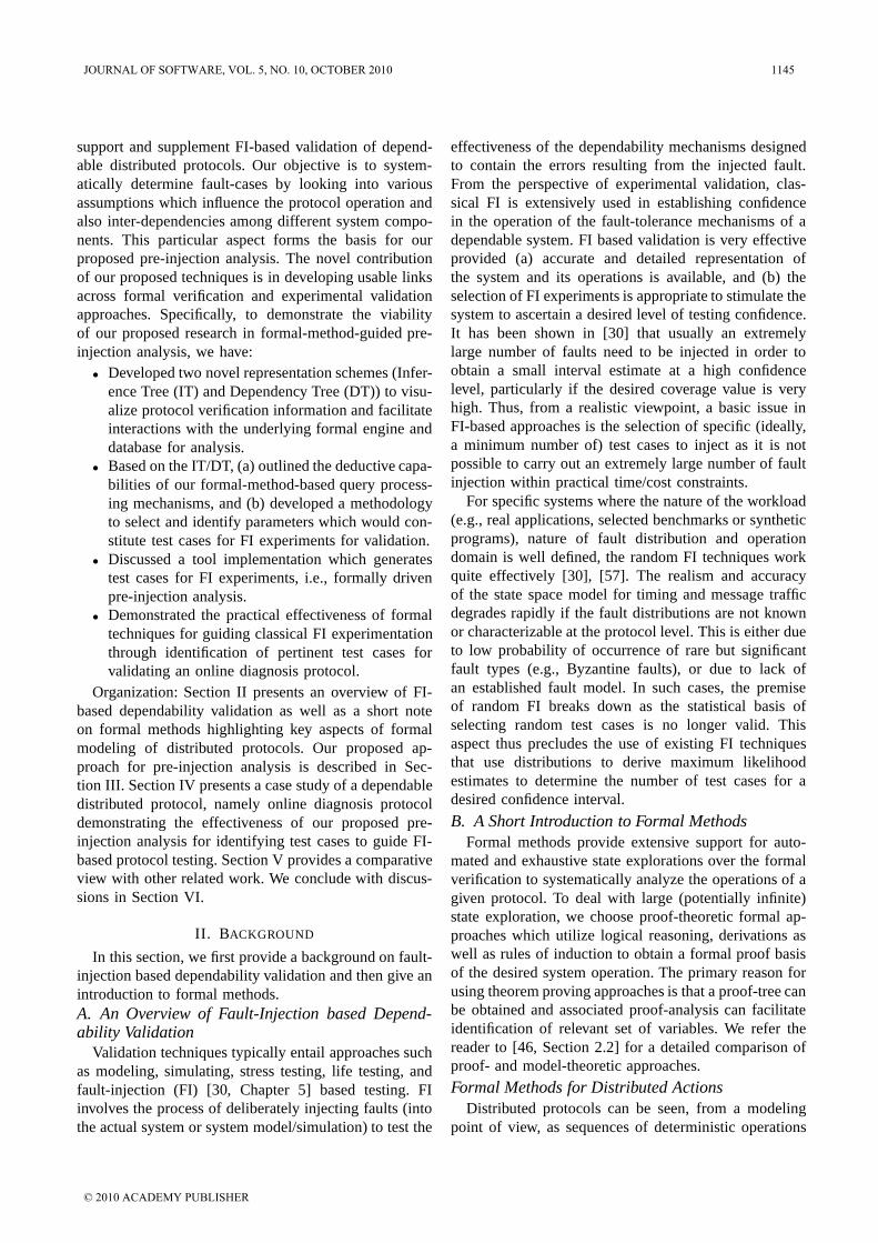
support and supplement FI-based validation of depend-able distributed protocols. Our objective is to system-atically determine fault-cases by looking into variousassumptions which influence the protocol operation andalso inter-dependencies among different system compo-nents. This particular aspect forms the basis for ourproposed pre-injection analysis. The novel contributionof our proposed techniques is in developing usable linksacross formal verification and experimental validationapproaches. Specifically, to demonstrate the viabilityof our proposed research in formal-method-guided pre-injection analysis, we have:

• Developed two novel representation schemes (Infer-ence Tree (IT) and Dependency Tree (DT)) to visu-alize protocol verification information and facilitateinteractions with the underlying formal engine anddatabase for analysis.

• Based on the IT/DT, (a) outlined the deductive capa-bilities of our formal-method-based query process-ing mechanisms, and (b) developed a methodologyto select and identify parameters which would con-stitute test cases for FI experiments for validation.

• Discussed a tool implementation which generatestest cases for FI experiments, i.e., formally drivenpre-injection analysis.

• Demonstrated the practical effectiveness of formaltechniques for guiding classical FI experimentationthrough identification of pertinent test cases forvalidating an online diagnosis protocol.

Organization: Section II presents an overview of FI-based dependability validation as well as a short noteon formal methods highlighting key aspects of formalmodeling of distributed protocols. Our proposed ap-proach for pre-injection analysis is described in Sec-tion III. Section IV presents a case study of a dependabledistributed protocol, namely online diagnosis protocoldemonstrating the effectiveness of our proposed pre-injection analysis for identifying test cases to guide FI-based protocol testing. Section V provides a comparativeview with other related work. We conclude with discus-sions in Section VI.

II. BACKGROUND

In this section, we first provide a background on fault-injection based dependability validation and then give anintroduction to formal methods.A. An Overview of Fault-Injection based Depend-ability Validation

Validation techniques typically entail approaches suchas modeling, simulating, stress testing, life testing, andfault-injection (FI) [30, Chapter 5] based testing. FIinvolves the process of deliberately injecting faults (intothe actual system or system model/simulation) to test the

effectiveness of the dependability mechanisms designedto contain the errors resulting from the injected fault.From the perspective of experimental validation, clas-sical FI is extensively used in establishing confidencein the operation of the fault-tolerance mechanisms of adependable system. FI based validation is very effectiveprovided (a) accurate and detailed representation ofthe system and its operations is available, and (b) theselection of FI experiments is appropriate to stimulate thesystem to ascertain a desired level of testing confidence.It has been shown in [30] that usually an extremelylarge number of faults need to be injected in order toobtain a small interval estimate at a high confidencelevel, particularly if the desired coverage value is veryhigh. Thus, from a realistic viewpoint, a basic issue inFI-based approaches is the selection of specific (ideally,a minimum number of) test cases to inject as it is notpossible to carry out an extremely large number of faultinjection within practical time/cost constraints.

For specific systems where the nature of the workload(e.g., real applications, selected benchmarks or syntheticprograms), nature of fault distribution and operationdomain is well defined, the random FI techniques workquite effectively [30], [57]. The realism and accuracyof the state space model for timing and message trafficdegrades rapidly if the fault distributions are not knownor characterizable at the protocol level. This is either dueto low probability of occurrence of rare but significantfault types (e.g., Byzantine faults), or due to lack ofan established fault model. In such cases, the premiseof random FI breaks down as the statistical basis ofselecting random test cases is no longer valid. Thisaspect thus precludes the use of existing FI techniquesthat use distributions to derive maximum likelihoodestimates to determine the number of test cases for adesired confidence interval.

B. A Short Introduction to Formal MethodsFormal methods provide extensive support for auto-

mated and exhaustive state explorations over the formalverification to systematically analyze the operations of agiven protocol. To deal with large (potentially infinite)state exploration, we choose proof-theoretic formal ap-proaches which utilize logical reasoning, derivations aswell as rules of induction to obtain a formal proof basisof the desired system operation. The primary reason forusing theorem proving approaches is that a proof-tree canbe obtained and associated proof-analysis can facilitateidentification of relevant set of variables. We refer thereader to [46, Section 2.2] for a detailed comparison ofproof- and model-theoretic approaches.

Formal Methods for Distributed ActionsDistributed protocols can be seen, from a modeling

point of view, as sequences of deterministic operations



interleaved with branching points, where the Function(or algorithm) takes decisions based on the actual infor-mation it has obtained. We can call such sequences ofdeterministic operations as Actions. In a proof-theoreticcontext1 we can prove the fact that an action implementsthe specified behavior as a theorem. That is, for eachaction we can try to build a proof that, starting fromsome given axioms or Conditionals certain Inferencescan be drawn out, which correspond to the possibility ofoperations, assertions, and/or usage of event conditionalvariables. Each action, being deterministically defined,can be modeled as a set of predicates. Using thesepredicates, we can try to prove certain conjectures (i.e.,unproven theorem) starting form the conditions given ashypothesis. Using the resulting inferences, it is possibleto determine: (a) which alternative branch will be chosenafter an action completes; (b) which are the conditionsfor the next action; (c) whether the protocol implementsthe specified and desired properties.

PVS Tool SupportAt the protocol level, the need is to be able to support

hierarchical operations and hierarchical decompositionof functional blocks. Thus, a high-level logic whichcan facilitate such a decomposition structure is required.For our studies, we used SRI’s Prototype VerificationSystem (PVS) tool [40] for our research, although ourapproaches are applicable to any higher order logic basedformal environment. PVS provides a powerful interactiveproof-checker with the ability to store and replay proofs.The PVS system provides several commands for deter-mining the status of theories, such as whether a proofhas been performed/completed. Proof-chain analysis, animportant form of status report, assures that all the proofobligations are fulfilled. It also identifies the axiomaticfoundation of the given theorem, i.e., it analyzes a givenproof to determine its dependencies.

III. PROPOSED PRE-INJECTION ANALYSIS

Formal methods have primarily been used as verifica-tion techniques (i.e., to capture conformance to designspecification) in establishing correctness of the design.On the other hand, experimental testing targets actualimplementations. Obviously a gap exists to transcendfrom abstract properties to implementation details. Thisresearch aims at bridging the gap between formal verifi-cation and experimental validation/testing. Towards thisaim, our key contributions include development of:

1An axiomatic theory consists of a number of primitive terms and setof statements which are true within that theory (known as axioms). Aproof in a theory is a finite sequence S1, S2, S3, . . . , Sn of statementsin the theory such that each S is an axiom, or can be derived fromany of the preceding statements by applying a rule of inference (suchstatements are known as theorems).

• A methodology for pre-injection analysis whichinvolves techniques for representation and visual-ization of verification information to establish thedependency of operations on specific variables asrepresented in formal specification of the proto-col. Moreover, the developed techniques providemechanisms for modifying parameters, variablesand decision operations to enumerate the relevantexecution paths of the protocol. This is achievedby updating the formal specification of the protocoland verifying the properties of interests through theunderlying formal-tool .

• An approach for identification/creation of suitableand specific FI test cases. It is achieved by utilizingrepresentation of execution paths as well as prop-agation paths depicting the scope of influence ofparameters and variables on the protocol operations.

Before describing the proposed methodology forformal-methods driven FI-based validation process, itis necessary to briefly introduce the two key structuredverification-information representation schemes.

A. Representation and Visualization of VerificationInformation

Typically, after developing the formal specification ofa protocol and its subsequent formal verification, theinformation at the verification stage is in the form ofmathematical logic in a syntax appropriate to the chosenformal tool-set. As our interest is in protocol validation,we need to transform and utilize the information gen-erated by the specification and verification process toaid the identification of system states, and to be able totrack the influence path of a variable or implementationparameter to construct a FI test case. Towards thisobjective, we have developed two structured represen-tation and visualization schemes to encapsulate variousinformation attributes. We label them as (a) InferenceTree (IT) or “forward propagation implication tree”, and(b) Dependency Tree (DT) or “backward propagationdeductive tree”. An IT outlines the inference conditionsand the actions taken during the verification process,while a DT captures the variable/functional block thatthe protocol/specification rely on. Moreover, DT facili-tates query processing and/or ‘what-if’ analysis on theinformation accumulated over the verification process.We present some basic features of these structures priorto discussing their complementary use in validation.

We observe that most dependable protocols consist ofdecision stages leading to branches processing specificerror-handling cases [5], [10], [19], [20], [54]. This is akey concept behind validation, which tries to investigateall the possible combinations of branching over time andwith parametric information (examples include numericbounds for variables, round number, processor attributes,



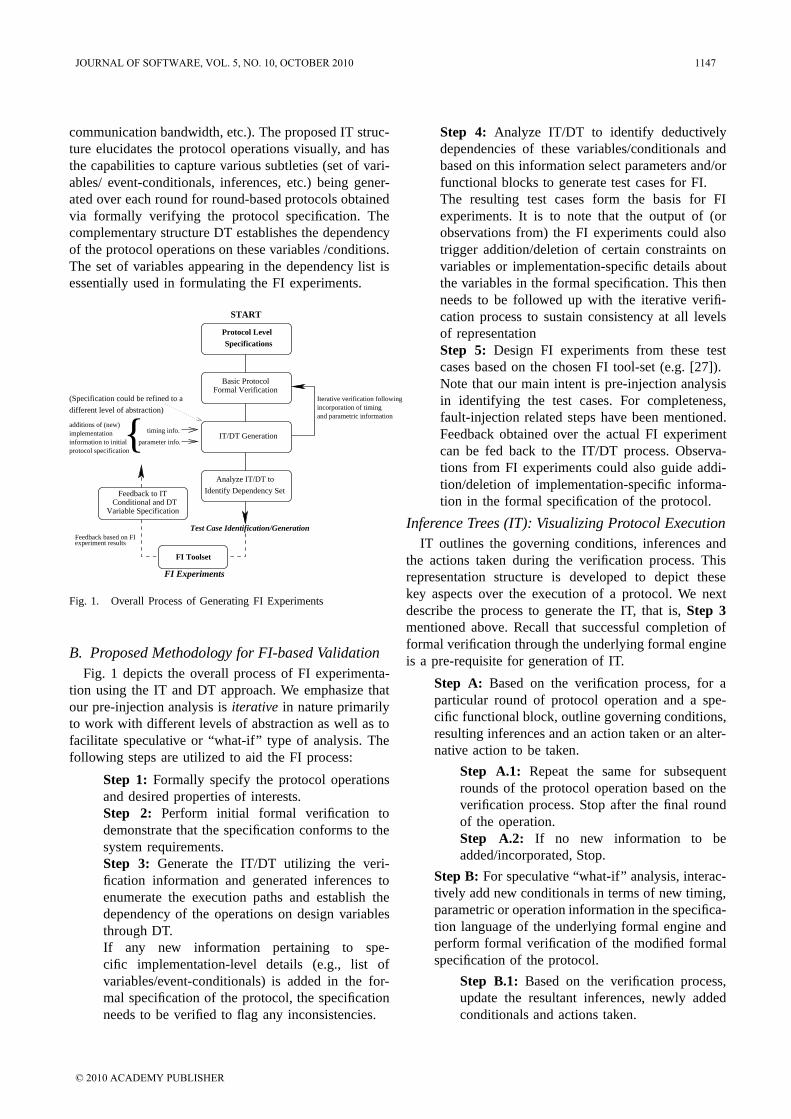
communication bandwidth, etc.). The proposed IT struc-ture elucidates the protocol operations visually, and hasthe capabilities to capture various subtleties (set of vari-ables/ event-conditionals, inferences, etc.) being gener-ated over each round for round-based protocols obtainedvia formally verifying the protocol specification. Thecomplementary structure DT establishes the dependencyof the protocol operations on these variables /conditions.The set of variables appearing in the dependency list isessentially used in formulating the FI experiments.

experiment resultsFeedback based on FI

different level of abstraction)

FI Experiments

START

(Specification could be refined to a

Protocol LevelSpecifications

Feedback to IT

Variable Specification

Basic ProtocolFormal Verification

IT/DT Generationtiming info.

parameter info.

Conditional and DT

Analyze IT/DT to

Identify Dependency Set

Test Case Identification/Generation

FI Toolset

Iterative verification followingincorporation of timingand parametric information

implementationinformation to initialprotocol specification

additions of (new)

Fig. 1. Overall Process of Generating FI Experiments

B. Proposed Methodology for FI-based ValidationFig. 1 depicts the overall process of FI experimenta-

tion using the IT and DT approach. We emphasize thatour pre-injection analysis is iterative in nature primarilyto work with different levels of abstraction as well as tofacilitate speculative or “what-if” type of analysis. Thefollowing steps are utilized to aid the FI process:

Step 1: Formally specify the protocol operationsand desired properties of interests.Step 2: Perform initial formal verification todemonstrate that the specification conforms to thesystem requirements.Step 3: Generate the IT/DT utilizing the veri-fication information and generated inferences toenumerate the execution paths and establish thedependency of the operations on design variablesthrough DT.If any new information pertaining to spe-cific implementation-level details (e.g., list ofvariables/event-conditionals) is added in the for-mal specification of the protocol, the specificationneeds to be verified to flag any inconsistencies.

Step 4: Analyze IT/DT to identify deductivelydependencies of these variables/conditionals andbased on this information select parameters and/orfunctional blocks to generate test cases for FI.The resulting test cases form the basis for FIexperiments. It is to note that the output of (orobservations from) the FI experiments could alsotrigger addition/deletion of certain constraints onvariables or implementation-specific details aboutthe variables in the formal specification. This thenneeds to be followed up with the iterative verifi-cation process to sustain consistency at all levelsof representationStep 5: Design FI experiments from these testcases based on the chosen FI tool-set (e.g. [27]).Note that our main intent is pre-injection analysisin identifying the test cases. For completeness,fault-injection related steps have been mentioned.Feedback obtained over the actual FI experimentcan be fed back to the IT/DT process. Observa-tions from FI experiments could also guide addi-tion/deletion of implementation-specific informa-tion in the formal specification of the protocol.

Inference Trees (IT): Visualizing Protocol ExecutionIT outlines the governing conditions, inferences and

the actions taken during the verification process. Thisrepresentation structure is developed to depict thesekey aspects over the execution of a protocol. We nextdescribe the process to generate the IT, that is, Step 3mentioned above. Recall that successful completion offormal verification through the underlying formal engineis a pre-requisite for generation of IT.

Step A: Based on the verification process, for aparticular round of protocol operation and a spe-cific functional block, outline governing conditions,resulting inferences and an action taken or an alter-native action to be taken.

Step A.1: Repeat the same for subsequentrounds of the protocol operation based on theverification process. Stop after the final roundof the operation.Step A.2: If no new information to beadded/incorporated, Stop.

Step B: For speculative “what-if” analysis, interac-tively add new conditionals in terms of new timing,parametric or operation information in the specifica-tion language of the underlying formal engine andperform formal verification of the modified formalspecification of the protocol.

Step B.1: Based on the verification process,update the resultant inferences, newly addedconditionals and actions taken.



Step B.2: If no new information to beadded/incorporated, Stop.

Step C: Iterate Step B for each new condition beingintroduced.

We first present a generic description of the IT andthen follow up with detailing different aspects of itthrough a specific case study. Please refer to Figure 2to relate the terms described next. Each node of thetree represents a primitive FUNCTION (or a functionalblock/ an algorithmic step of the protocol) at a givenlevel of abstraction. Associated with each node is a setof CONDITIONALS (assumptions specified as axiomsin the formal specification) which dictate the flow of op-eration to the subsequent ACTION(s) as defined for theprotocol. Also associated with each node is the INFER-ENCES space which details the possibility of operation(or sequence of operations), assertions, and/or usage ofevent-conditional variables which can be inferred fromthe node/operation specification. A particular inferencecould potentially update the conditionals for the subse-quent round of protocol execution where a specific actionwill be taken. Note that FUNCTION, CONDITIONALS,INFERENCES and ACTION are constituent part of theIT structure. Furthermore, a connection (edge) betweentwo nodes/functional blocks represents a logical or tem-poral relation in terms of algorithmic actions/steps takenbased on the prevailing conditions. A path between twonodes comprising of multiple connections represents aset of actions taken up by the protocols.

The set of CONDITIONALS consists of two parts:(i) the basic algorithm (definitions), assumptions, andconstraints, and (ii) postulated properties (claims) aboutthe protocol. Thus, initially, the CONDITIONAL spacecontains only the basic assumptions and constraintsfor the given protocol, and basic derivative proper-ties. Over subsequent verification rounds, the CONDI-TIONAL space is enhanced with more information aboutparameters that may impact the behavior of the protocol.Note that both CONDITIONALS and INFERENCES areformally obtained from the protocol specifications. Infact the theorem prover process defines the conditionalsas requisite stopping conditions to be satisfied prior toproceeding to a subsequent step in a proof. Using func-tional level specification of the protocol, an IT representsthe complete set of activation paths of the protocol (i.e.,enumeration of all operations). It is important to pointout that the process of generating CONDITIONAL andINFERENCE spaces are semi-automatic and involvesusers intuitions and understanding of formal specifica-tion, and the implications of the proofs. Moreover, itis notable that both CONDITIONAL and INFERENCEspaces can grow or shrink depending on the protocol andits operating conditions, though the growth of these two

spaces are linearly bounded by the system parameters.In order to keep track of influences of newly added

conditionals on the protocol operation, the IT structurefacilitates recording of inference(s) leading to specificaction(s) (we label them as “leads to this action”) aswell as resulting inference(s) updating the conditionalsfor the subsequent round of protocol execution (we labelthem as “updates . . . operation”).

Another key feature of the IT is that it provides formixed levels of abstraction, as a function block can berepresented as a complete graph by itself. For example,the voter function can be represented at the circuit levelabstraction and modeled in say RTL-level specificationas shown in Fig. 2 (the lower right-most node).

An Illustration of the Inference Tree – Example of the2/3 Majority Voter

After having given a generic description of the IT, weillustrate the development of the inference tree throughan example of a majority voter. Consider a triple modularredundant (TMR) system, where three process repli-cas produce results for a voter to generate a majorityresponse. Request ordering is a critical issue, that is,we want all replicas to process the same sequence ofrequests. One way to handle this is to allow each clientto attach a timestamp to each request. Another key issuein the voter is that of vote synchronization, i.e., ensuringthat the tabulated result is based on a set of votes thatare all responses to the same request. Communicationdelays or other problems may prevent some votes fora particular request from reaching the voter in a timelymanner. As we do not impose any constraints on thevoter itself, the voter must rely on other information forsynchronization. Moreover, a voting session takes placewhenever there are sufficient number of votes for a givenfailure class (e.g., fail-stop) for a particular request. If areplica’s vote misses its intended voting round, the voteis treated as an obsolete vote.

Fig. 2 represents the generation of an IT for a majority(2/3) voter. Each node of the tree represents a primitiveFUNCTION (or functional block of the protocol) at agiven level of abstraction. Here, FUNCTION is the 2/3voter, i.e., 2 out of 3 nodes need to agree for a result.

Further, in Fig. 2, a set of CONDITIONALS C[· · · ]describes the various conditions (actual or speculative)imposed on the voter. As examples, C[T ime Window]indicates a condition that a message will be processedby the voter only if it arrives in a specified time window,say [t − ∆, t + ∆], C[Sequence] indicates the conditionon the sequence of message arrival, C[Count] denotesthe number of votes received for a particular round, andC[Round] imposes constraints that all the messages are



Count_LowNo_Majority

repeating round # n)

Leads to thisaction

Initial Information

C[Org_Condof round #n]

Leads to thisaction

round # n

round # n

for the next round of operationUpdates the conditional space

New/added Info.

Alternate flow of operation

Actual flow of operation

Resulting inference leads to an action

Resulting inference updates/adds a condition

New Information to CONDITIONAL space

Incoming message A functional specification of a protocol operation

A functional specification at a different

Operating condition

t(...)?(...)

C[...]Operating condition being true

Operating condition NOT being true

level of abstraction

New/added Info.

(Sufficient number of vote counts;Majority found)

round # n+1

incoming messages (votes)functional levelspecification

t(Majority)

(Insufficient number of vote counts;Majority not found)

ACTION: Declare Error(if no majority is found after

?(Count)

?(Majority)CONDITIONALS

INFERENCES

FUNCTION

ACTION: Repeat operation for round # n

ACTION: Proceed for round #n+1

FUNCTION

C[Count]C[Sequence]

C[Round]

INFERENCES

C[Voter_Rate]

2/3 voter

C[Time_Window]

(e.g., RTL level of specification))(Can be specified at a varied level of abstraction

FUNCTION

2/3 voter

2/3 voter

LEGENDS

CONDITIONALS

t(Sequence) t(Time_Window)t(Round)

Fig. 2. The Inference Tree for a 2/3 Voter Protocol

from the same round n. Based on the inputs to thevoter and the governing conditions mentioned above,specific ACTIONS such as the voter outputs a result (andproceeds to the next round) or a repeat of the votingprocess, and corresponding operational INFERENCESare generated. In the INFERENCE space, t(Round)denotes that the condition C[Round] is true whereas?(Count) reflects the fact that the condition C[Count]is not satisfied.

Based on inferences, a specific action is taken. Theseresulting inferences in turn get reflected in the CONDI-TIONAL space of the IT depicting information for thenext round of operation, to govern the subsequent roundsof protocol operation. In Fig. 2, we also highlight whichinference(s) leads to which action(s) (depicted witharrows labeled “leads to this action”) as well as whichresulting inference(s) causes updating of the conditionalsfor the subsequent round of protocol execution (depictedby arrows labeled “updates . . . operation”). Note thatbased on the prior inference (first instance of round #n) of C[Count] not being satisfied, during the secondinstance (repeat) of round # n if sufficient number ofvotes are not received, then an action such as “DeclareError” could be taken. C[Org Cond of round # n]

captures all the conditions that were imposed during thefirst instance of round # n.

ACTIONS are protocol-related. For example, for a 2/3voter as depicted in Fig. 2, we outline two potential AC-TIONS that could be taken after round # n. If a sufficientnumber of votes and all other related conditions weresatisfied, the voter proceeds with the next round of votingprocess, otherwise, the voter may repeat the operation forround # n. These can be considered as branching pointswhere the protocol takes a decision based on informationit has gathered.

A novel property of the IT structure is that it allowsfor refinements in specification. Initially, the IT represen-tation is at the protocol level. Over subsequent iterations,parametric/implementation information is added. For ex-ample, in Fig. 2, in the CONDITIONAL space of the ITdepicting the second instance of round # n activities,a condition C[V oter Rate], indicating TMR voting rateto be greater than or equal to the message input rate, canbe added as an implementation detail (beyond the tradi-tional descriptions of TMR) to the specification. As newconditional or parametric information is incorporated, acomplete verification (and inference) cycle is performedto highlight any inconsistency the new parameters might



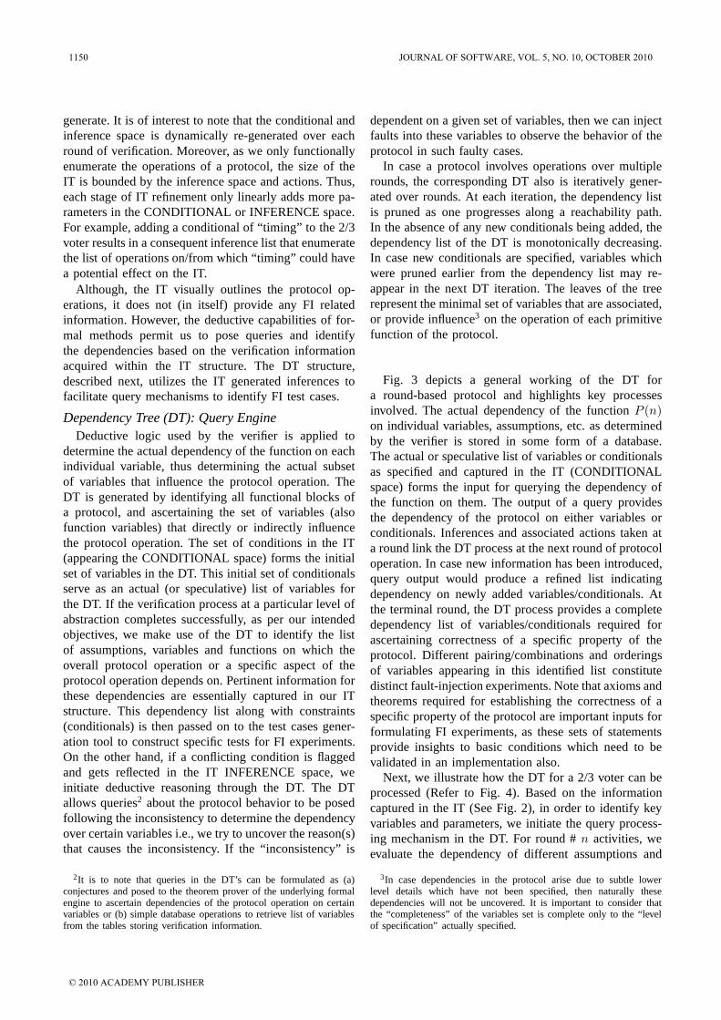
generate. It is of interest to note that the conditional andinference space is dynamically re-generated over eachround of verification. Moreover, as we only functionallyenumerate the operations of a protocol, the size of theIT is bounded by the inference space and actions. Thus,each stage of IT refinement only linearly adds more pa-rameters in the CONDITIONAL or INFERENCE space.For example, adding a conditional of “timing” to the 2/3voter results in a consequent inference list that enumeratethe list of operations on/from which “timing” could havea potential effect on the IT.

Although, the IT visually outlines the protocol op-erations, it does not (in itself) provide any FI relatedinformation. However, the deductive capabilities of for-mal methods permit us to pose queries and identifythe dependencies based on the verification informationacquired within the IT structure. The DT structure,described next, utilizes the IT generated inferences tofacilitate query mechanisms to identify FI test cases.

Dependency Tree (DT): Query EngineDeductive logic used by the verifier is applied to

determine the actual dependency of the function on eachindividual variable, thus determining the actual subsetof variables that influence the protocol operation. TheDT is generated by identifying all functional blocks ofa protocol, and ascertaining the set of variables (alsofunction variables) that directly or indirectly influencethe protocol operation. The set of conditions in the IT(appearing the CONDITIONAL space) forms the initialset of variables in the DT. This initial set of conditionalsserve as an actual (or speculative) list of variables forthe DT. If the verification process at a particular level ofabstraction completes successfully, as per our intendedobjectives, we make use of the DT to identify the listof assumptions, variables and functions on which theoverall protocol operation or a specific aspect of theprotocol operation depends on. Pertinent information forthese dependencies are essentially captured in our ITstructure. This dependency list along with constraints(conditionals) is then passed on to the test cases gener-ation tool to construct specific tests for FI experiments.On the other hand, if a conflicting condition is flaggedand gets reflected in the IT INFERENCE space, weinitiate deductive reasoning through the DT. The DTallows queries2 about the protocol behavior to be posedfollowing the inconsistency to determine the dependencyover certain variables i.e., we try to uncover the reason(s)that causes the inconsistency. If the “inconsistency” is

2It is to note that queries in the DT’s can be formulated as (a)conjectures and posed to the theorem prover of the underlying formalengine to ascertain dependencies of the protocol operation on certainvariables or (b) simple database operations to retrieve list of variablesfrom the tables storing verification information.

dependent on a given set of variables, then we can injectfaults into these variables to observe the behavior of theprotocol in such faulty cases.

In case a protocol involves operations over multiplerounds, the corresponding DT also is iteratively gener-ated over rounds. At each iteration, the dependency listis pruned as one progresses along a reachability path.In the absence of any new conditionals being added, thedependency list of the DT is monotonically decreasing.In case new conditionals are specified, variables whichwere pruned earlier from the dependency list may re-appear in the next DT iteration. The leaves of the treerepresent the minimal set of variables that are associated,or provide influence3 on the operation of each primitivefunction of the protocol.

Fig. 3 depicts a general working of the DT fora round-based protocol and highlights key processesinvolved. The actual dependency of the function P (n)on individual variables, assumptions, etc. as determinedby the verifier is stored in some form of a database.The actual or speculative list of variables or conditionalsas specified and captured in the IT (CONDITIONALspace) forms the input for querying the dependency ofthe function on them. The output of a query providesthe dependency of the protocol on either variables orconditionals. Inferences and associated actions taken ata round link the DT process at the next round of protocoloperation. In case new information has been introduced,query output would produce a refined list indicatingdependency on newly added variables/conditionals. Atthe terminal round, the DT process provides a completedependency list of variables/conditionals required forascertaining correctness of a specific property of theprotocol. Different pairing/combinations and orderingsof variables appearing in this identified list constitutedistinct fault-injection experiments. Note that axioms andtheorems required for establishing the correctness of aspecific property of the protocol are important inputs forformulating FI experiments, as these sets of statementsprovide insights to basic conditions which need to bevalidated in an implementation also.

Next, we illustrate how the DT for a 2/3 voter can beprocessed (Refer to Fig. 4). Based on the informationcaptured in the IT (See Fig. 2), in order to identify keyvariables and parameters, we initiate the query process-ing mechanism in the DT. For round # n activities, weevaluate the dependency of different assumptions and

3In case dependencies in the protocol arise due to subtle lowerlevel details which have not been specified, then naturally thesedependencies will not be uncovered. It is important to consider thatthe “completeness” of the variables set is complete only to the “levelof specification” actually specified.



various operational constraints. Generated via a Test Case Generation Tool

P(n)

P(n+1)

Inferences/Action link the two nodes

Input: Speculative or actual list of axioms/theorems.Query: Depends on which assumptions?

Input: Speculative or actual list of variable definitionsQuery: Depends on which variable definitions?

Output: Refined output list is produced indicating

dependency (or lack of it) on newly incorporated

P(m)

axioms, theorems required for establishing correctness

of a specific property.

Output: List of dependent variables over round # nOutput: List of dependent axioms/theoremsobtained from the IT CONDITIONALS space obtained from the IT CONDITIONALS space

A complete dependency list of variable definitions,

P: a round−based protocol

and assumption added in the specs.New timing/parametric information

Terminal round

variable definitions/axioms/theorems over round # n+1

FI Experiment: Combinations of "variable−value" pairs out of the dependency list satisfying

Fig. 3. The Dependency Tree : Highlights of Key Processes Involved in a Round-based Protocol

variable definitions by parsing the information generatedover the verification process. In Fig. 4, predicate voted?returns true if the given replica voted, vote ok? returnstrue if the vote is not obsolete, and fail-stop maj ok?returns true if sufficient non-obsolete votes are there forfinding majority. Note that the DT points out that thechosen implementation of the 2/3 majority voter doesnot depend on C[Sequence]. For other fault-tolerant ma-jority voting schemes such as a function which discardstop k and bottom k values and then takes the medianof the remaining values, the correctness of such a voterdepends on the sequencing of the requests as governedby C[Sequence].

We emphasize that the DT may not fully representall possible variable dependencies as it will alwaysbe limited to the amount of operational informationactually modeled into the formal specification. At anydesired level, the elements of the current dependency listprovides us with a (possibly) minimal set of parameterswhich should help formulate the FI experiments via allpermutations and combinations, and ideally should gen-erate specific (or a family of) test cases. We repeat thatour intent is pre-injection analysis in identifying specifictest cases. The actual FI experiments are implementedfrom these test cases based on the chosen FI tool-set(s).C. Overall Process of Identifying the Influential Setof Protocol Variables/Conditions

In order to realize our proposed methodology forpre-injection analysis, we have used PVS specifica-tion language to specify the protocol operation and its

theorem prover to establish the correctness of variousproperties of interests. The construction of IT/DT andsubsequent analysis in the DT as discussed earlier isessentially carried out by exploiting the information thatgets generated as part of verification process. The deriveddependency-list gets stored in the DT and subsequentlyused to perform certain queries for pre-injection analysis.

In order to prune the list of variables (and in turnstate-space associated with them), we compare the listprovided by the DT process with the actual or speculativelist of variables/conditional specified in the IT. Utilizingthe DT information and comparison results, we iden-tify the redundant variables and/or conditionals speci-fied/used in the initial specification of the protocol. Theseredundant variables (those variables that are specified butare not influencing in anyway the protocol operation)are then eliminated from the IT CONDITIONAL spaceand the verification process is repeated again to ensurethat the specification and the corresponding verificationare consistent and up-to-date. Next, test cases for an FIexperiment for a chosen tool-set can be constructed usingthe identified minimal set of variables.D. Generation of Test Suites for Fault-Injection Ex-periments

In order to support the test generation aspect of ourproposed methodology, we have developed a tool calledSampurna [56] which generates a comprehensive set oftest suites by eliminating the variable-value pairs thatare not attainable/possible with respect to the protocolspecification by using a priori knowledge of the system.The concept of cross product is introduced to capture allthe possible combination of variables so as to generate



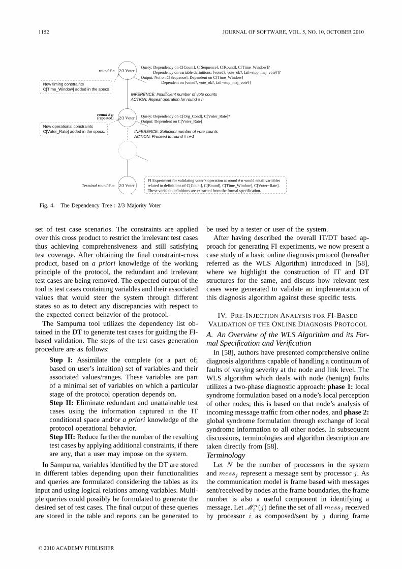
round # n

2/3 Voter

2/3 Voter

2/3 VoterFI Experiment for validating voter’s operation at round # n would entail variablesrelated to definitions of C[Count], C[Round], C[Time_Window], C[Voter−Rate].These variable definitions are extracted from the formal specification.

ACTION: Repeat operation for round # nINFERENCE: Insufficient number of vote counts

Dependency on variable definitions: [voted?, vote_ok?, fail−stop_maj_vote?]?Output: Not on C[Sequence]; Dependent on C[Time_Window]

Dependent on [voted?, vote_ok?, fail−stop_maj_vote?]

INFERENCE: Sufficient number of vote countsNew operational constraintsC[Voter_Rate] added in the specs.

New timing constraintsC[Time_Window] added in the specs

Terminal round # m

round # nQuery: Dependency on C[Count], C[Sequence], C[Round], C[Time_Window]?

ACTION: Proceed to round # n+1

Output: Dependent on C[Voter_Rate]Query: Dependency on C[Org_Cond], C[Voter_Rate]?(repeated)

Fig. 4. The Dependency Tree : 2/3 Majority Voter

set of test case scenarios. The constraints are appliedover this cross product to restrict the irrelevant test casesthus achieving comprehensiveness and still satisfyingtest coverage. After obtaining the final constraint-crossproduct, based on a priori knowledge of the workingprinciple of the protocol, the redundant and irrelevanttest cases are being removed. The expected output of thetool is test cases containing variables and their associatedvalues that would steer the system through differentstates so as to detect any discrepancies with respect tothe expected correct behavior of the protocol.

The Sampurna tool utilizes the dependency list ob-tained in the DT to generate test cases for guiding the FI-based validation. The steps of the test cases generationprocedure are as follows:

Step I: Assimilate the complete (or a part of;based on user’s intuition) set of variables and theirassociated values/ranges. These variables are partof a minimal set of variables on which a particularstage of the protocol operation depends on.Step II: Eliminate redundant and unattainable testcases using the information captured in the ITconditional space and/or a priori knowledge of theprotocol operational behavior.Step III: Reduce further the number of the resultingtest cases by applying additional constraints, if thereare any, that a user may impose on the system.

In Sampurna, variables identified by the DT are storedin different tables depending upon their functionalitiesand queries are formulated considering the tables as itsinput and using logical relations among variables. Multi-ple queries could possibly be formulated to generate thedesired set of test cases. The final output of these queriesare stored in the table and reports can be generated to

be used by a tester or user of the system.After having described the overall IT/DT based ap-

proach for generating FI experiments, we now present acase study of a basic online diagnosis protocol (hereafterreferred as the WLS Algorithm) introduced in [58],where we highlight the construction of IT and DTstructures for the same, and discuss how relevant testcases were generated to validate an implementation ofthis diagnosis algorithm against these specific tests.

IV. PRE-INJECTION ANALYSIS FOR FI-BASED

VALIDATION OF THE ONLINE DIAGNOSIS PROTOCOL

A. An Overview of the WLS Algorithm and its For-mal Specification and Verification

In [58], authors have presented comprehensive onlinediagnosis algorithms capable of handling a continuum offaults of varying severity at the node and link level. TheWLS algorithm which deals with node (benign) faultsutilizes a two-phase diagnostic approach: phase 1: localsyndrome formulation based on a node’s local perceptionof other nodes; this is based on that node’s analysis ofincoming message traffic from other nodes, and phase 2:global syndrome formulation through exchange of localsyndrome information to all other nodes. In subsequentdiscussions, terminologies and algorithm description aretaken directly from [58].Terminology

Let N be the number of processors in the systemand messj represent a message sent by processor j. Asthe communication model is frame based with messagessent/received by nodes at the frame boundaries, the framenumber is also a useful component in identifying amessage. Let M n

i (j) define the set of all messj receivedby processor i as composed/sent by j during frame



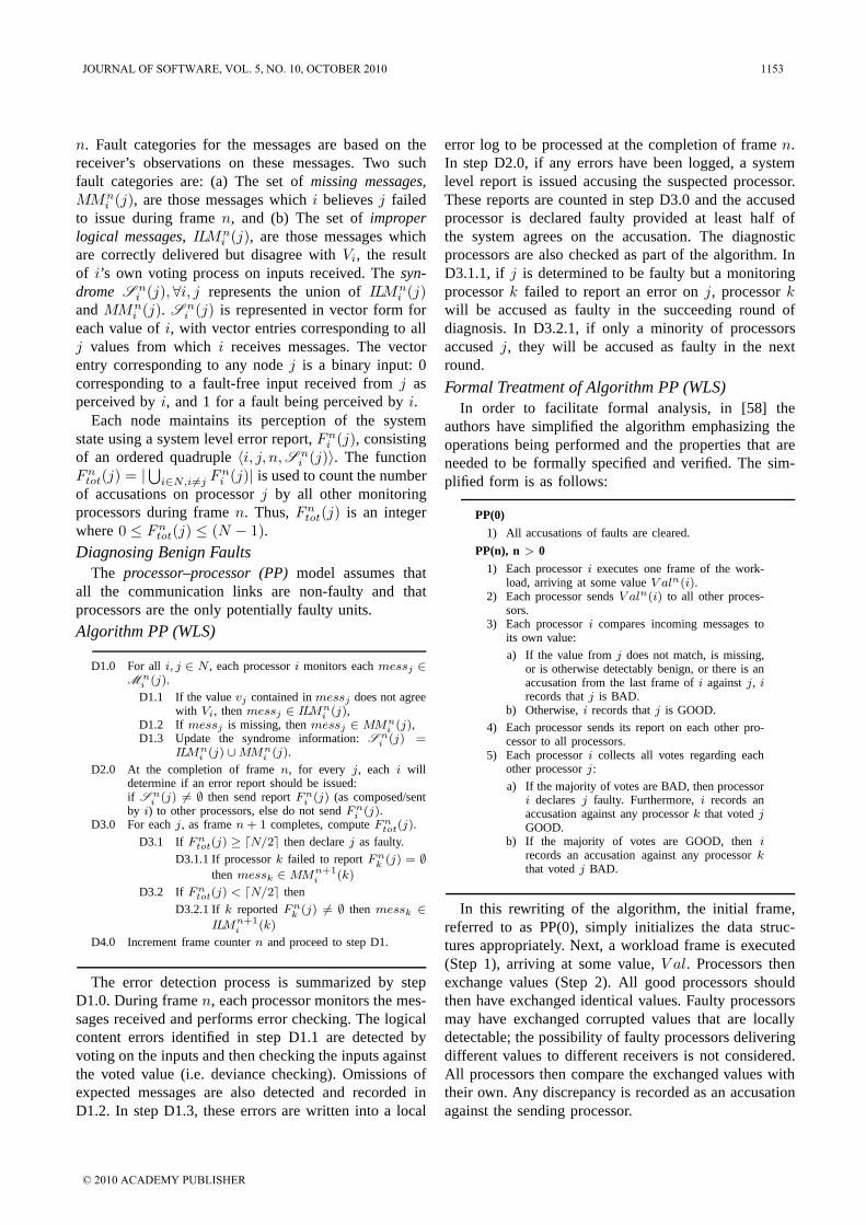
n. Fault categories for the messages are based on thereceiver’s observations on these messages. Two suchfault categories are: (a) The set of missing messages,MMn

i (j), are those messages which i believes j failedto issue during frame n, and (b) The set of improperlogical messages, ILMn

i (j), are those messages whichare correctly delivered but disagree with Vi, the resultof i’s own voting process on inputs received. The syn-drome S n

i (j), ∀i, j represents the union of ILMni (j)

and MMni (j). S n

i (j) is represented in vector form foreach value of i, with vector entries corresponding to allj values from which i receives messages. The vectorentry corresponding to any node j is a binary input: 0corresponding to a fault-free input received from j asperceived by i, and 1 for a fault being perceived by i.

Each node maintains its perception of the systemstate using a system level error report, Fn

i (j), consistingof an ordered quadruple 〈i, j, n, S n

i (j)〉. The functionFn

tot(j) = |⋃

i∈N,i=j Fni (j)| is used to count the number

of accusations on processor j by all other monitoringprocessors during frame n. Thus, Fn

tot(j) is an integerwhere 0 ≤ Fn

tot(j) ≤ (N − 1).

Diagnosing Benign FaultsThe processor–processor (PP) model assumes that

all the communication links are non-faulty and thatprocessors are the only potentially faulty units.

Algorithm PP (WLS)

D1.0 For all i, j ∈ N , each processor i monitors each messj ∈M n

i (j).

D1.1 If the value vj contained in messj does not agreewith Vi, then messj ∈ ILMn

i (j),D1.2 If messj is missing, then messj ∈ MMn

i (j),D1.3 Update the syndrome information: S n

i (j) =ILMn

i (j) ∪ MMni (j).

D2.0 At the completion of frame n, for every j, each i willdetermine if an error report should be issued:if S n

i (j) = ∅ then send report F ni (j) (as composed/sent

by i) to other processors, else do not send F ni (j).

D3.0 For each j, as frame n + 1 completes, compute F ntot(j).

D3.1 If F ntot(j) ≥ N/2 then declare j as faulty.

D3.1.1 If processor k failed to report F nk

(j) = ∅

then messk ∈ MMn+1

i (k)

D3.2 If F ntot(j) < N/2 then

D3.2.1 If k reported F nk

(j) = ∅ then messk ∈

ILMn+1

i (k)

D4.0 Increment frame counter n and proceed to step D1.

The error detection process is summarized by stepD1.0. During frame n, each processor monitors the mes-sages received and performs error checking. The logicalcontent errors identified in step D1.1 are detected byvoting on the inputs and then checking the inputs againstthe voted value (i.e. deviance checking). Omissions ofexpected messages are also detected and recorded inD1.2. In step D1.3, these errors are written into a local

error log to be processed at the completion of frame n.In step D2.0, if any errors have been logged, a systemlevel report is issued accusing the suspected processor.These reports are counted in step D3.0 and the accusedprocessor is declared faulty provided at least half ofthe system agrees on the accusation. The diagnosticprocessors are also checked as part of the algorithm. InD3.1.1, if j is determined to be faulty but a monitoringprocessor k failed to report an error on j, processor kwill be accused as faulty in the succeeding round ofdiagnosis. In D3.2.1, if only a minority of processorsaccused j, they will be accused as faulty in the nextround.

Formal Treatment of Algorithm PP (WLS)In order to facilitate formal analysis, in [58] the

authors have simplified the algorithm emphasizing theoperations being performed and the properties that areneeded to be formally specified and verified. The sim-plified form is as follows:

PP(0)

1) All accusations of faults are cleared.

PP(n), n > 0

1) Each processor i executes one frame of the work-load, arriving at some value V aln(i).

2) Each processor sends V aln(i) to all other proces-sors.

3) Each processor i compares incoming messages toits own value:

a) If the value from j does not match, is missing,or is otherwise detectably benign, or there is anaccusation from the last frame of i against j, i

records that j is BAD.b) Otherwise, i records that j is GOOD.

4) Each processor sends its report on each other pro-cessor to all processors.

5) Each processor i collects all votes regarding eachother processor j:

a) If the majority of votes are BAD, then processori declares j faulty. Furthermore, i records anaccusation against any processor k that voted j

GOOD.b) If the majority of votes are GOOD, then i

records an accusation against any processor k

that voted j BAD.

In this rewriting of the algorithm, the initial frame,referred to as PP(0), simply initializes the data struc-tures appropriately. Next, a workload frame is executed(Step 1), arriving at some value, V al. Processors thenexchange values (Step 2). All good processors shouldthen have exchanged identical values. Faulty processorsmay have exchanged corrupted values that are locallydetectable; the possibility of faulty processors deliveringdifferent values to different receivers is not considered.All processors then compare the exchanged values withtheir own. Any discrepancy is recorded as an accusationagainst the sending processor.



Developing the Formal Specification of PPThe formal specification of PP is specified in a single

PVS theory called pp. In the theory pp, some otherpredefined theories are explicitly imported4. This theorytakes several parameters which include m, the maximumnumber of periods, n, the number of processors, andT , the type values that are passed between processors.The term error represents values that are benign uponlocal receipt, such as missing values, values failing paritycheck, values failing digital signature checks, and so on.BAD and GOOD are the values of accusations sent byprocessors over the network. Finally, the function Val isassumed to return the correct value for each frame ofcomputation, and that the correct value is never any ofthe special values error, BAD, or GOOD.

The type statuses is defined to be an enumeration ofthree constants, corresponding to three of the categoriesof behavior: symmetric-value faulty, benign, and good.The function status returns the status of a given processor(or fault containment unit fcu).

Some notations are used for describing statuses: s,c, and g are predicates recognizing the symmetric-value faulty, benign, and good processors, respectively.Similarly, given a set caucus, as(caucus) is the set ofarbitrary-faulty processors in caucus. The functions ss,cs and gs similarly select the symmetric-value faulty,benign, and good processors, respectively.

The function send captures the properties of sendingvalues from one processor to another. This function takesa value to be sent, a sender, and a receiver as arguments;it returns the value that would be received if the receiverwere a good processor. The behavior of send is axiom-atized according to the status of the sender. The firstaxiom simply says that a good processor sends correctvalues to all (good) receivers: g(p) ⊃ send(t,p,q)= t.The second axiom says that a benign faulty processoralways delivers values that are recognized as erroneousby good receivers: c(p) ⊃ send(t,p,q) = error. Thethird axiom says that a symmetric-value faulty processorsends the same value to all good receivers, althoughthat value is otherwise unconstrained (i.e., it may beany possible value, including those that are recognizedas erroneous) s(p) ⊃send(t,p,q) = send(t,p,z). Nothingis specified for the behavior of asymmetric-value faultysenders. A lemma (called send5) is stated and provedthat all receivers obtain the same value no matter whatthe status of the sender (here, the possibility of link andarbitrary faults is discounted) send(t,p,q) = send(t,p,z).

The function HybridMajority is intended to be similarto the standard Majority function, except that all errorvalues are excluded. The function HybridMajority takes

4The complete theory specification adapted from [58] is presentedin the Appendix.

two arguments, a set of processors (i.e., an fcuset), whichwe call the caucus, and a vector mapping processorsto values (i.e., an fcuvector). Several properties relatedto HybridMajority that are of particular interests aredescribed below:

The first property states that if the vector recordsthe same non-error value for all good processors inthe caucus, and the vector records an error value forall benign-faulty (benign) processors in the caucus, andthere are more good processors than symmetric-valuefaulty processors in the caucus, then HybridMajorityreturns the same value as that recorded in the vectorfor the good processors.

The second property states that the value returneddepends only on the values recorded in the vector forthe processors in the caucus.

The final property deals with the fact that if thereare more good than symmetric-faulty processors and allgood processors agree on some non-error value, and theHybridMajority function returns a value, then that valueis the value of each good processor.

Next, the definition of some of the key functions ofthe actual algorithm is discussed.

Syndrome(R,j,i,OldAccuse):T =IF OldAccuse(i,j) OR (NOT Val(R)=send(Val(R),j,i)) THEN BAD

ELSE GOODENDIF

The Syndrome function above is meant to capture theproperty that in period R, i believes j is faulty. Theparameter OldAccuse essentially records old accusationsfrom earlier periods. The only other reason to accusea processor of faulty behavior is if that processor sentsome value that does not correspond to the correct value.The next function KDeclareJ (i.e., k declares j faulty)is built using the Syndrome function. The definition is:

KDeclareJ(pset,R,OldAccuse,j,k):bool=HybridMajority(pset, LAMBDA i:send(Syndrome(R,j,i,OldAccuse),i,k))=BAD

This predicate is meant to capture the idea thatprocessor k will gather all accusations against someprocessor j, and then take the HybridMajority of thatset. If most processors accuse j, then this predicate istrue, i.e., k declares j faulty. The main function, for“processor-processor model” based diagnostic algorithm,PP is specified below:

PP(pset,R,OldAccuse)(i,j):RECURSIVE bool =IF R=0 THEN FALSEELSE KDeclareJ(pset,R,OldAccuse,j,i) ORPP(pset, R-1, (lambda i2,k: OldAccuse(i2,k) OREXISTS j2:(KDeclareJ(pset,R,OldAccuse,j2,i2)/=(send(Syndrome(R,j2,k,OldAccuse),k,i2)=BAD))))(i,j)

ENDIF MEASURE (LAMBDA pset, R, OldAccuse : R)

The intended meaning of this formal description isthat after R periods, starting with OldAccuse accusations,



processor i believes that processor j is faulty. Thefunction PP is defined as a recursive function. If thenumber of periods R is zero, then i will not accusej. If KDeclareJ(pset,R,OldAccuse,j,i), that is, if aftergathering votes for period R, a (hybrid) majority of otherprocessors send i an accusation of j, then i believes jis faulty. Otherwise, PP is called recursively, using oneless period. The recursive call also updates OldAccuse toinclude the case that some processor misdiagnosed someother processor. That is, an accusation is added to thelocal OldAccuse for the next period if the voted diagnosisKDeclareJ(pset,R,OldAccuse,j2,i2) of some processor j2does not agree with the individual accusation sent fromk to i2.

The two properties dealing with soundness and com-pleteness are formally specified and verified using PVSin [58]. We have added (and at places modified) a fewspecifications as needed. The first requirement that ofSoundness states if the algorithm PP declares a processorto be faulty, then it is indeed faulty. The key propertyaddressed here is that all good processors accuse onlyfaulty processors of being faulty. Essentially, we wantto prove that if i is good, and after R periods of PP,i accuses j, then either j is benign or symmetric-valuefaulty. The second property, Completeness, states that ifa processor is faulty, then PP will determine this.B. Visualization: IT/DT for the WLS Fault-Diagnosis Algorithm

The formal verification of the two properties statedabove is based on the prove-by-induction on the numberof rounds. The PVS tool allows the user to conductpartial proofs under different assumptions and specialcases of interests.

The objective of the formal verification and repre-sentation of verification information in the IT structureis to guide the selection of appropriate queries to beposed in the DT. It is important to note that the selectionand formal representation of queries to be posed is stillan interactive process. This is typical for any theoremproving (proof theoretic) environment where the user’sknowledge of the specified protocol activities guides theprocess of query formulation. Note that for both IT andDT, we describe them in simple English as depicting theinformation in the formal syntax of PVS would not beappropriate for general readers.Development of the IT Structure

In Fig. 5, we depict the operational flow of the PP(WLS) algorithm for a particular node for three roundsof activities starting with round # n. The initial set ofconditionals on which the protocol operation begins withis listed below.

• g(p) → send(t, p, q) = t

• c(p) → send(t, p, q) = error• s(p) → send(t, p, q) = send(t, p, z)

• send(t, p, q) = send(t, p, z)• ∀p : g(p) ∧ p ∈ caucus → v(p) = t ∧ t = error [A ]• ∀p : c(p) ∧ p ∈ caucus → v(p) = error [B]• ‖caucus‖ = ‖cs(caucus)‖+‖ss(caucus)‖+‖gs(caucus)‖• ‖gs(caucus)‖ > ‖ss(caucus)‖ ∧ A ∧ B → HybridMajor-

ity(caucus, v) = t

• N ≥ 3 and E < N/2 where N and E are the total numberof nodes and the number of faulty nodes, respectively.

• Syndromeni (j) = BAD → ¬(V aln(j) =

send(V aln(j), j, i)) ∨ OldAccuse(i, j)

As a general rule, to guide the proof process toproceed in a desired way, we add conditions as the proof-steps are taken. For processor i to judge processor j inround # n, it looks at either the value sent by processorj (i.e., send(V aln(j), j, i)) or an old accusation aboutprocessor j (i.e., OldAccuse). By setting the predicateOldAccuse(i,j) to be true, we let the function PP to returntrue by setting the predicate KDeclareJ to true over theround # n +1. KDeclareJ being true indicates that aftern rounds, starting with OldAccuse accusations, processori believes that processor j is faulty.

Similarly, for a processor k to be declared faulty byprocessor i over round # n + 2 as it could not diagnoseprocessor j to be faulty as majority of processors diddeclare j to be a faulty processor, in the recursive partof PP with one less round (i.e., for round # R-1), thesecond clause (that is, EXISTS j2... appearing in asnippet of formal specification of PP ) need to be set truein order to update OldAccuse to reflect that processor kmisdiagnosed processor j.

We now describe the IT for the WLS algorithmdepicting the operational flow for a node ‘i’ in the system(See Fig. 5). The ways of triggering or setting variousconditions to steer the flow of protocol operation havebeen discussed in the preceding paragraphs. During theexecution over round n, node i receives a message fromnode j and also a syndrome of j from node x as preparedby it after round # n−1. C[Set] in the CONDITIONALSspace reflects the initial set of conditions. Over roundn, based on the value received from node j and asyndrome from node x reflecting that it suspects j tobe faulty, node i suspects j to be faulty, informs othernodes about its assessment and then proceeds to thenext round. These inferences have been captured in theINFERENCES space. They in turn update the CONDI-TIONALS space for the next round (n+1) and also leadto the specific action of recording j ‘BAD’ and sendinga report. Based on the notations introduced in Fig. 2,we have highlighted these in Fig. 5 with arrows labeled“Updates...” and “Leads to...”, respectively. Over round #n+1, based on the reports from other nodes about nodej after round n, node i collates this information andperforms the majority voting. If the majority of nodes



INFERENCES

Reports from other nodes about ’j’

PP

PP

PP

i

i

iround # n

round # n+2

CONDITIONALS

CONDITIONALS

INFERENCES

INFERENCES

CONDITIONALS

Message from node ’j’

round # n+1

for round # n

Reports from other nodes about ’k’

Majority voted’k’ faulty

’i’ declares ’k’faulty

’x’ suspected

’i’ records ’j’

Majority voted’j’ faulty

’k’ finds ’j’non−faulty

’i’ declares ’j’faulty

BAD’i’ records ’k’

BAD

after round # n

after round # n+1

Syndrome of ’j’ from

node ’x’ after round # n−1

C[Set]: Initial set of Conditionalsas listed in the text.

C[Set]

C[Set]

’i’ suspects ’j’faulty ’j’ faulty

Updates Conditionals spacefor the next round

for the next roundUpdates Conditionals space

Leads to this action

Leads to this action

ACTION: Record ’k’ BAD and send report

ACTION: Record ’j’ GOOD and send report

ACTION: Record ’j’ BAD and send report

Fig. 5. The IT for the WLS Online Diagnosis Algorithm – Operational Flow Illustrated for Node ‘i’

voted node j to be faulty, then node i also declaresnode j to be faulty. If a node k fails to find j faulty,then node i prepares a syndrome for node k and sendsthat to other nodes. Over round # n + 2, based onthe reports from other nodes about node k after roundn + 1, node i collates this information and performs themajority voting. If majority of nodes found node k tobe faulty, then node i also declares node k to be faulty.In the event, if one of the conditions were not satisfied,alternate actions could have been taken as marked inFig. 5.

Development of the DT StructureIn Fig. 6, we illustrate how the DT of the WLS

algorithm can be processed. Based on the informationcaptured in the IT (Fig. 5), in order to identify key vari-ables and conditionals, we initiate the query processingin the DT. For round n activities, we determine the actualand lack of dependency on the conditionals/variables aslisted in the CONDITIONAL space of the IT. At eachiteration, the dependency list is pruned as one progressesover multiple rounds of protocol execution. Moreover,in case new conditionals are specified, variables whichwere pruned earlier from the dependency list may re-appear in the next iteration. As illustrated in Fig. 6,round n of the protocol operation does not dependon assumption HybridMajority, however, upon addingtimeout as a new condition for the subsequent rounds ofoperation, the assumption HybridMajority re-appears inthe dependency list for rounds # n+1 and n+2. Belowwe highlight the complete list of dependencies for the

completeness property PP (i.e., if a processor is faulty,then the PP will determine this) to hold.

Dependency List: s, g, c, gs, cc, ss, send1, send2,PP, Empty, HybridMajority, KDeclareJ, Syndrome,OldAccuse

FI experiments for validating the PP (WLS) algo-rithm at rounds n, n+1 and n+2 would entail variablesrelated to the definition of the terms listed above. Weprovide further details on this aspect in Section IV-Cwhere we discuss validation of a Java implementationof the WLS algorithm.

C. Validation of a Java Implementation of the WLSAlgorithm

We have implemented the online diagnosis algorithm(PP) in Java. A requirement was that a user can verify ifa processor was declared as being faulty by monitoringthe outputs on the command line. Instead of a processorreceiving values for a workload and computing majorityto obtain a value, we decided that each node would sendonly one value per frame. This helps in determiningwhen to end a frame, as we would wait for a definedtime period in order to receive messages from all theother processors in the network. Also, as per the originaldescription of the algorithm if there were no errors thenthere would be no error reports sent. However, there isno specification on how long a processor should wait foran error report. So, we included a timeout so that errorreports received before the timeout would be processed



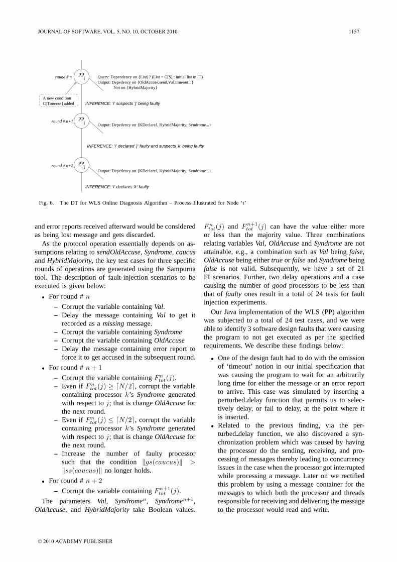
A new condition

PP

iPP

iPP

INFERENCE: ’i’ suspects ’j’ being faulty

INFERENCE: ’i’ declared ’j’ faulty and suspects ’k’ being faulty

round # n+2

round # n+1

round # n

Output: Depedency on KDeclareJ, HybridMajority, Syndrome...

Output: Depedency on KDeclareJ, HybridMajority, Syndrome...

Query: Dependency on List? (List = C[S] : initial list in IT)Output: Depedency on OldAccuse,send,Val,timeout...

Not on HybridMajority

INFERENCE: ’i’ declares ’k’ faulty

C[Timeout] added

i

Fig. 6. The DT for WLS Online Diagnosis Algorithm – Process Illustrated for Node ‘i’

and error reports received afterward would be consideredas being lost message and gets discarded.

As the protocol operation essentially depends on as-sumptions relating to sendOldAccuse, Syndrome, caucusand HybridMajority, the key test cases for three specificrounds of operations are generated using the Sampurnatool. The description of fault-injection scenarios to beexecuted is given below:

• For round # n

– Corrupt the variable containing Val.– Delay the message containing Val to get it

recorded as a missing message.– Corrupt the variable containing Syndrome– Corrupt the variable containing OldAccuse– Delay the message containing error report to

force it to get accused in the subsequent round.

• For round # n + 1

– Corrupt the variable containing Fntot(j).

– Even if Fntot(j) ≥ N/2, corrupt the variable

containing processor k’s Syndrome generatedwith respect to j; that is change OldAccuse forthe next round.

– Even if Fntot(j) ≤ N/2, corrupt the variable

containing processor k’s Syndrome generatedwith respect to j; that is change OldAccuse forthe next round.

– Increase the number of faulty processorsuch that the condition ‖gs(caucus)‖ >‖ss(caucus)‖ no longer holds.

• For round # n + 2

– Corrupt the variable containing Fn+1tot (j).

The parameters Val, Syndromen, Syndromen+1,OldAccuse, and HybridMajority take Boolean values.

Fntot(j) and Fn+1

tot (j) can have the value either moreor less than the majority value. Three combinationsrelating variables Val, OldAccuse and Syndrome are notattainable, e.g., a combination such as Val being false,OldAccuse being either true or false and Syndrome beingfalse is not valid. Subsequently, we have a set of 21FI scenarios. Further, two delay operations and a casecausing the number of good processors to be less thanthat of faulty ones result in a total of 24 tests for faultinjection experiments.

Our Java implementation of the WLS (PP) algorithmwas subjected to a total of 24 test cases, and we wereable to identify 3 software design faults that were causingthe program to not get executed as per the specifiedrequirements. We describe these findings below:

• One of the design fault had to do with the omissionof ‘timeout’ notion in our initial specification thatwas causing the program to wait for an arbitrarilylong time for either the message or an error reportto arrive. This case was simulated by inserting aperturbed delay function that permits us to selec-tively delay, or fail to delay, at the point where itis inserted.

• Related to the previous finding, via the per-turbed delay function, we also discovered a syn-chronization problem which was caused by havingthe processor do the sending, receiving, and pro-cessing of messages thereby leading to concurrencyissues in the case when the processor got interruptedwhile processing a message. Later on we rectifiedthis problem by using a message container for themessages to which both the processor and threadsresponsible for receiving and delivering the messageto the processor would read and write.



• Another interesting case that revealed the deficiencyin our implementation was that we had missed outthe checking of the processor’s health to determinewhether it is a healthy or faulty processor. Attimes, in our system the number of faulty processorswould be more than the good or healthy processorsand still we would perform majority and take thevotes of faulty processors to get a majority vote.This sometimes led to declaration of a healthyprocessor as a faulty in a caucus of three processors.From our viewpoint, this case would not havebeen identified via classical testing techniques. Thisbecame a trivial test to conduct as the dependencylist included terms gs and ss, and the condition‖gs(caucus)‖ > ‖ss(caucus)‖ was also capturedin the IT conditional space.

DiscussionsFormal methods require the right mix of effort, ex-

pertise, and knowledge. In this particular case study,we leveraged from the work already done as part ofthe development of online diagnosis algorithms [58].However, in our other case studies [51], [49], substantialefforts (about 1 man-year) were put in developing theformal specification and subsequently verifying desiredproperties of the protocols used therein. It is importantto emphasize that nowadays protocols developed forhighly dependable systems typically go through formalverification, and it would be ideal to exploit (and reusein a meaningful way) the information generated overthe verification process to guide the validation of animplementation of that protocol.

V. COMPARATIVE VIEW WITH RELATED WORK

The classical use of formal methods has been forthe verification of protocols, and specifically, on findingdesign stage flaws in the protocols. In [6], the focusof the work is on the verification of fault-toleranceproperties using model-based formalisms, specifically anexecutable specification has been developed to establishthe tolerated behavior of the spacecraft computers inpresence of faults. In literature, a variety of approacheshave developed excellent concepts in linking formal ap-proaches to testing (See [2], [4], [7], [8], [12], [16], [23],[28], [29], [35], [39], [52], [55], [60] among others).While there has been a lot of work on specification-basedtesting and test case generation [15], [22], not muchwork has focused on bridging the gap between theoremproving and testing. In [13], authors have presentedthe HOL-TestGen system that generates unit tests fromIsabelle specifications. In [9], a tool that uses HOLspecifications for testing protocols has been discussed.In [41], the author has presented strategies to createrandom test cases directly from PVS [40] specifications.

In particular, to the best of our knowledge, the keydistinction of our approach from others is that we makeprominent use of proof-theoretic-based reasoning, andlink/analyze the inferences generated over the verifica-tion process to determine key assumptions and the setof (implementation) parameters to derive scenarios todrive FI experiments. Though our approach is proof-theoretic, we could potentially utilize (and interface)model theoretic approaches as well. In [45], the authorshave developed a unified framework to provide supportfor both proof-theoretic as well as model-theoretic ap-proaches. As mentioned in Section III-B, our approachallows for mixed level of abstraction. For example, at thecircuit level abstract, a function can be modeled in sayRTL-level specification. Such a low-level abstraction ofthe program is useful to reason about hardware errors.The formal model can then be rigorously analyzed undererror conditions against the above specifications usingtechniques such as model checking and theorem proving.

Existing efforts [1], [5], [10], [16], [18], [19], [21],[53], [54] have explored deterministic approaches fortest case identification for validation. The work reportedin [16], [19], [21] have exploited some typical propertiesof fault tolerant protocols (e.g., decision stages, chainof furcated fault-handling actions, etc.) for modelingcomplex distributed protocols. Our proposed representa-tion schemes share properties with other state-transitionrepresentations like assertion trees [5], [54] or Petrinets [20]. We point out that [20] uses a formal speci-fication of the protocol and it is processed using someheuristic to identify influence parameters in an automatedmanner. In particular, reachability analysis is performedto identify fault cases and their corresponding activationpaths. In order to reduce the size of the reachabilitygraph certain restrictions on the protocol behavior isassumed. This scheme works well for bounded systems,however, for protocols dealing with real-time and non-deterministic attributes, this approach is limited.

Similar to our proposed approach, the work reportedin [33] presents a symbolic approach for injecting faults(those relating to HW errors only) into programs writtenin Java and considers the effect of bit-flips in programvariables. However, HW errors which can alter the con-trol flow of the program have not been considered by thetechnique. In [44], the authors have presented a programlevel framework that allows specification of arbitrarydetectors and their verification against transient HWerrors using symbolic execution and model checking.In a recent paper [26], the authors have proposed aframework for generating test vectors from specificationswritten in the Prototype Verification System (PVS) [40].The methodology uses a translator to produce a Javaprototype from a PVS specification. Symbolic (Java)



PathFinder [43] is then employed to generate a collectionof test cases. The combination of these two existing toolsenables this process by automating much of the task.

VI. CONCLUSIONS, SUMMARIZING PAST WORK AND

FUTURE DIRECTIONS

The conventional FI approaches are facing growinglimitations in handling the large state space involvedin the operations of dependable distributed and real-time protocols. We have shown the efficacy of formaltechniques as an supplement for FI-based validationof dependable distributed protocols that have a formalspecification and whose models have been validated. Inthis paper, we have applied our approach to an onlinediagnosis algorithm and illustrated the effectiveness ofthe proposed pre-injection analysis in identifying rele-vant though critical test cases against which an imple-mentation of the diagnosis protocol must be validated.

In [51], we introduced the basic idea of using formalmethods for pre-injection analysis to derive a set ofparameters to describe fault-injection scenarios. With thecase study of clock synchronization [51], we highlightedthe following key capabilities of our proposed pre-injection analysis approach: (a) support for traceabil-ity of fault-propagation over different functional block,(b) identification of a specific functional block whichneed to be further examined depending upon the infer-ences captured (via IT) and corresponding dependencylist generated (via DT) for that block, and (c) support formodeling (or incorporating specification) of a specificfunctional block at a refined level of abstraction. Overthis case study we also demonstrated the capabilitiesof IT/DT approaches to pinpoint a specific block (e.g.,2/3 Voter) which needed to be modeled to identify thecause of a failure (partial ordering problem of messagesarriving at a specific node). In this case, 3827 tests wereneeded using classical FI versus 24 tests identified by ourproposed approach. In both cases, the implementationhad 3 fault cases and both techniques were correctlyable to identify them. The identified parametric attributesinclude: round number, concurrency time-window, vot-ing rate and numeric range for message sequences. Itis to note that such information resulting over a pre-injection analysis facilitate (or guide) intelligent waysof determining influential (or key) variables to generateFI experiments for validating protocol operations.

In [49], [50], we demonstrated the effectiveness andefficiency of our approaches through the example ofFT clock synchronization and FT Rate Monotonic Al-gorithm (FT-RMA) [25]. In the case of the fault-tolerant real-time task scheduling algorithm namely FT-RMA [49], [50], we were able to identify flaws in theanalysis, and using IT/DT obtain the specific conditionsto constitute effective FI test cases which, in fact,

confirmed our identification of flaws. As a comparativeanalysis of our proposed pre-injection analysis techniquewith conventional approaches, we showed that eventhough FT-RMA protocols had gone through extensivesimulation and random FI experiments, fault cases be-longing to one of our derived equivalence classes of faulttypes were not identified. Typically, for simulations, tasksets are randomly generated and due to their limitationsin considering factors involving key schedulability crite-ria, these task sets would have a low probability to coverall key aspects of fault-tolerance and timing issues whichwe were able to capture during the formal treatment ofpre-injection analysis of FT-RMA protocols.

Though the formal approach for analysis appears tobe very attractive and effective, it has its own limi-tations. The foremost limitation is in the capabilitiesof formal techniques for representation of parametricattributes (e.g., specifying numeric bounds for variables,processor attributes, etc.), real-time deadlines, systemworkload conditions, etc. Furthermore, associated withthese attributes, the corresponding formal verificationprocess also needs to be developed. We have yet to fullyincorporate the specification of system load (and stress)into the formal engine. At present we are limited toapproximating these conditions using distributions; in thefuture we are looking at approaches to model stress andload as parametric inputs. We acknowledge that furtherenhancement of the proposed pre-injection analysis isrequired to broaden the applicability of the approach.

ACKNOWLEDGMENTS

We thank Peter Bokor and Marco Serafini for pro-viding constructive feedback on the paper. Researchsupported in part by EC Indexsys, Inspire, TUD CASEDand DFG GRK 1362 (TUD GKMM).

REFERENCES

[1] G.A. Alvarez, F. Cristian, “Cesium: Testing Hard Real-Time andDependability Properties of Distributed Protocols,” Proc. of IEEEWORDS’97, pg. 2–8, 1997.

[2] T. Amnell, et al., “Uppaal – Now, Next and Future,” Modellingand verification of Parallel Processes, LNCS – 2067, Springer-Verlag, pp. 100–125, 2001.

[3] J. Arlat, et al., “Fault Injection for Dependability Validation :A Methodology and Some Applications,” IEEE Trans. SoftwareEngineering, SE 16(2), pp. 166–182, Feb. 1990.

[4] A. Arnold et al., “An Experiment on the Validation of a Spec-ification by Heterogeneous Formal Means: The Transit Node.”Proc. of DCCA-5, pp. 24–34, 1995.

[5] D. Avresky, J. Arlat, J.-C. Laprie, Y. Crouzet, “Fault Injectionfor the Formal Testing of Fault Tolerance,” IEEE Trans. onReliability, vol. 45, pp. 443–455, 1996.

[6] S. Ayache, et al., “Formal Methods for the Validation of Fault-Tolerance in Autonomous Spacecraft,” IEEE FTCS-26, 1996.

[7] E. Bayse, A. Cavalli, M. Nunez, F. Zaidi, “A Passive Testing Ap-proach based on Invariants: Application to the WAP.” ComputerNetworks, 48(2), pp. 247-266, June 2005.

[8] G. Bernot, “Software Testing Based on Formal Specifications,”Software Engg. Journal, 6(6), pp. 387–405, Nov. 1991.



[9] S. Bishop, et al., “Rigorous Specification and Conformance Test-ing Techniques for Network Protocols, as Applied to TCP, UDP,and Sockets,” Proceedings of SIGCOMM 2005: ACM Conferenceon Computer Communications, published as Vol. 35, No. 4 ofComputer Communication Review, pp. 265–276, Aug. 2005.

[10] D.M. Blough, T. Torii, “Fault Injection Based Testing of FaultTolerant Algorithms in Message Passing Parallel Computers,”Proc. of FTCS-27, pp. 258–267, 1997.

[11] J. Boue, P. Petillon, Y. Crouzet, “MEFISTO-L: A VHDL-BasedFault Injection Tool for the Experimental Assessment of FaultTolerance,” Proc. of FTCS-28, pp. 168–173, 1998.

[12] E. Brinksma, “Formal Methods for Conformance Testing: TheoryCan be Practical,” CAV, LNCS 1639, pp. 44–46, 1999.

[13] A. Brucker, B. Wolf, “Test-Sequence Generation with HOL-TestGen - With an Application to Firewall Testing,” Tests andProofs, LNCS 4454.Springer-Verlag, 2007.

[14] R. Butler, G. Finelli, “The Infeasibility of Quantifying the Relia-bility of Life Critical Real Time Software,” IEEE Trans. SoftwareEngineering, SE 19(1), pp. 3–12, Jan. 1993.

[15] J. Chang, D. J. Richardson, “Structural Specification-based Test-ing: Automated Support and Experimental Evaluation,” Proceed-ings FSE99, pp. 285–302, Sept. 1999.

[16] W. Chen et al., “Model Checking Large SW Specifications,”IEEE Trans. SE, 7, pp. 498–520, July 1998.

[17] J. Christmansson, P. Santhaman, “Error Injection Aimed at FaultRemoval in Fault Tolerance Mechanisms – Criteria for ErrorSelection Using Field Data on Software Faults,” Proc. of ISSRE,pp. 175–184, 1996.

[18] S. Dawson, F. Jahanian, T. Mitton, T-L Tung, “Testing of Fault-Tolerant and Real-Time Distributed Systems via Protocol FaultInjection.” Proc. of FTCS–26, pp. 404–414, 1996.

[19] K. Echtle, et al. “Evaluation of Deterministic Fault Injection forFT Protocol Testing,” Proc. of FTCS-21, pp. 418–425, 1991.

[20] K. Echtle, M. Leu, “Test of FT Distributed Systems by FaultInjection,” FTPDS, pp. 244–251, 1995.

[21] K. Echtle, M. Leu, “The EFA Fault Injector for Fault-TolerantDistributed System Testing.” IEEE FTPDS, pp. 28–35, 1992.

[22] A. Gargantini, C. Heitmeyer, “Using Model Checking to Gen-erate Tests from Requirements Specifications,” Proc. of the 7thEuropean Eng. Conf. pp. 146–162. Springer-Verlag, 1999.

[23] M-C. Gaudel, “Testing Can be Formal Too?,” Proc. of TAPSOFT95, vol. 915, LNCS, pp. 82–96, May 1995.

[24] S. Ghosh, R. Melhem, D. Mosse, “Fault-Tolerant Rate MonotonicScheduling.” Proc. of DCCA–6, 1997.

[25] S. Ghosh, R. Melhem, D. Mosse, J.S. Sarma, “Fault-TolerantRate Monotonic Scheduling.” Real-Time Systems,, vol. 15, no. 2,pp. 149–181, Sept. 1998.

[26] A. Goodloe, C. Pasareanu, D. Bushnell, P. Miner, “A Test Gener-ation Framework for Distributed Fault-Tolerant Algorithms,” 4thWorkshop on Automated Formal Methods (AFM09), 2009.

[27] K.K. Goswami, R.K. Iyer, L. Young, “DEPEND: A Simulation-Based Environment for System Level Dependability Analysis,”IEEE Trans. on Computers, 46(1), pp. 60–74, Jan. 1997.

[28] W. Gujjahr et al., “Partition Testing vs. Random Testing: TheInfluence of Uncertainity,” IEEE Trans. on SE, pp. 661–674,Sept/Oct. 1999.

[29] L. Heerink et al., “Formal Test Automation: The Conf. Protocolwith Phact,” Proc. of Test Conf., pp. 211–220, 2000.

[30] R. Iyer, D. Tang, “Experimental Analysis of Computer SystemDependability,” Book chapter in ‘Fault Tolerant Computer SystemDesign’, editor: D.K. Pradhan, Prentice Hall, pp. 282–392, 1996.

[31] M. Joseph, Real-time Systems: Specification, Verification andAnalysis. Prentice Hall, London, 1996.

[32] J-C. Laprie, “Dependable Computing and Fault Tolerance: Con-cepts and Terminology.” FTCS-15, pp. 2–11, 1985.

[33] D. Larsson, R. Hahnle, “Symbolic Fault-Injection,” InternationalVerification Workshop (Verify), vol. 259, pp. 85–103, 2007.

[34] J. Lehoczky, L. Sha, Y. Ding, “The Rate Monotonic SchedulingAlgorithm: Exact Characterization and Average Case Behavior.”Proceedings of IEEE RTSS, pp. 166–171, December 1989.

[35] Yu Lei, D. Kung, Qizhi Ye, “A blocking-based approach to proto-col validation.” Computer Software and Applications Conference,COMPSAC 2005, pp. 301–306, July 2005.

[36] R.Lent, “A testbed validation tool for MANET implementations.”MASCOTS 2005, pp. 381–388, Sept. 2005.

[37] C.L. Liu, J.W. Layland, “Scheduling Algorithms for Multipro-gramming in a Hard-Real-Time Environment.” Journal of theACM, 20(1), pp. 46–61, January 1973.

[38] S. Mullender (Ed.), Distributed Systems, Addision-Wesley, 1993.[39] V. Okun, P.E. Black, Y. Yesha, “Testing with Model Checker:

Insuring Fault Visibility.” WSEAS Transactions, 2003.[40] S. Owre, J. Rushby, N. Shankar, F. von Henke, “Formal Verifica-

tion for Fault-Tolerant Architectures: Prolegomena to the Designof PVS,” IEEE Trans. Software Engineering, SE 21(2), pp. 107–125, February 1995.

[41] S. Owre, “Random Testing in PVS,” In Workshop on AutomatedFormal Methods, 2006.

[42] M. Pandya, M. Malek,“Minimum Achievable Utilization forFault-Tolerant Processing of Periodic Tasks,” IEEE Trans. onComputers, 47(10), pp. 1102–1112, Oct. 1998.

[43] C. Pasareanu, et al., “Combining Unit-Level Symbolic Executionand System-Level Concrete Execution for Testing NASA Soft-ware,” Proc. of Int. Symp. on SW Testing and Analysis, pp. 15–26.ACM Press, 2008.

[44] K. Pattabiraman, N. Nakka, Z. Kalbarczyk, R. Iyer, “Sym-PLFIED: Symbolic Program-Level Fault-Injection and Error-Detection Framework,” IEEE DSN, June 2008.

[45] S. Rajan, N. Shankar, M.K. Srivas, “An Integration of Model-Checking with Automated Proof Checking,” Computer-AidedVerification, CAV ’95, LNCS 939, pp. 84–97, 1995.

[46] J. Rushby, “Formal Methods and the Certification of CriticalSystems,” SRI-TR CSL-93-7, Dec. 1993.

[47] J. Rushby, F. von Henke, “Formal Verification of Algorithms forCritical Systems.” IEEE Trans. on SE, 19(1), pp. 13–23, 1993.

[48] M. Singhal, N.G. Shivaratri, Advanced Concepts in OperatingSystems, McGraw Hill, 1994.

[49] P. Sinha, N. Suri, “Identification of Test Cases Using a FormalApproach,” Proc. of FTCS–29, pp. 314–321, 1999.

[50] P. Sinha, N. Suri, “ On the Use of Formal Techniques forAnalyzing Dependable RT Protocols,” Proc. of RTSS, pp. 126–135, Dec. 1999.

[51] N. Suri, P. Sinha, “On the Use of Formal Techniques forValidation.” Proc. of FTCS-28, pp. 390–399, 1998.

[52] T. Suzuki et al., “Murate: A Protocol Modeling & VerificationApproach Based on a Specification language and Petri Nets,”IEEE Trans. on SE, SE 16, pp. 523–536, May 1990.

[53] S. Tao, et al., “Focused Fault Injection of Software ImplementedFault Tolerance Mechanisms of Voltan TMR Nodes.” DistributedSystems Engineering, 2(1), pp. 39–49, March 1995.

[54] T. Tsai, S.J. Upadhaya, H. Zhao, M.-C. Hsueh, R.K. Iyer, “Path-Based Fault Injection,” Proc. 3rd ISSAT Conf. on R&Q in Design,pp. 121–125, 1997.

[55] J. Tretmans, “Specification Based testing with Formal Methods:From Theory via Tools to Applications,” Proc. of FORTE 2000.

[56] N. Varma, et al., “CAGILY: An Approach for Developing TestSuites for Component-Based Systems,” IASTED SEA, Nov. 2003.

[57] J. Voas, G. McGraw, Software Fault Injection: Inoculating Pro-grams Against Errors, John Wiley & Sons Ltd, New York, 1998

[58] C.J. Walter, P. Lincoln, N. Suri, “Formally Verified On-LineDiagnosis” IEEE Trans. on Software Engg., Nov. 1997.

[59] W. Wang, et al., “The Impact of Fault Expansion on the IntervalEstimate for Fault Detection Coverage,” Proc. of FTCS–24, pp.330–337, 1994.

[60] Shu Xiao, et al., “Integrated TCP/IP Protocol Software Testingfor Vulnerability Detection.” ICCNMC, Oct. 2003.

Neeraj Suri holds the TUD Chair Professorshipat the Dept of CS, TU Darmstadt Germany. De-tails on his professional activities can be found athttp://www.deeds.informatik.tu-darmstadt.de/.

Purnendu Sinha is a Staff Researcher at GeneralMotors R&D, Bangalore, India. His research interestsinclude dependable distributed systems, software engi-neering, and formal-methods based V&V.



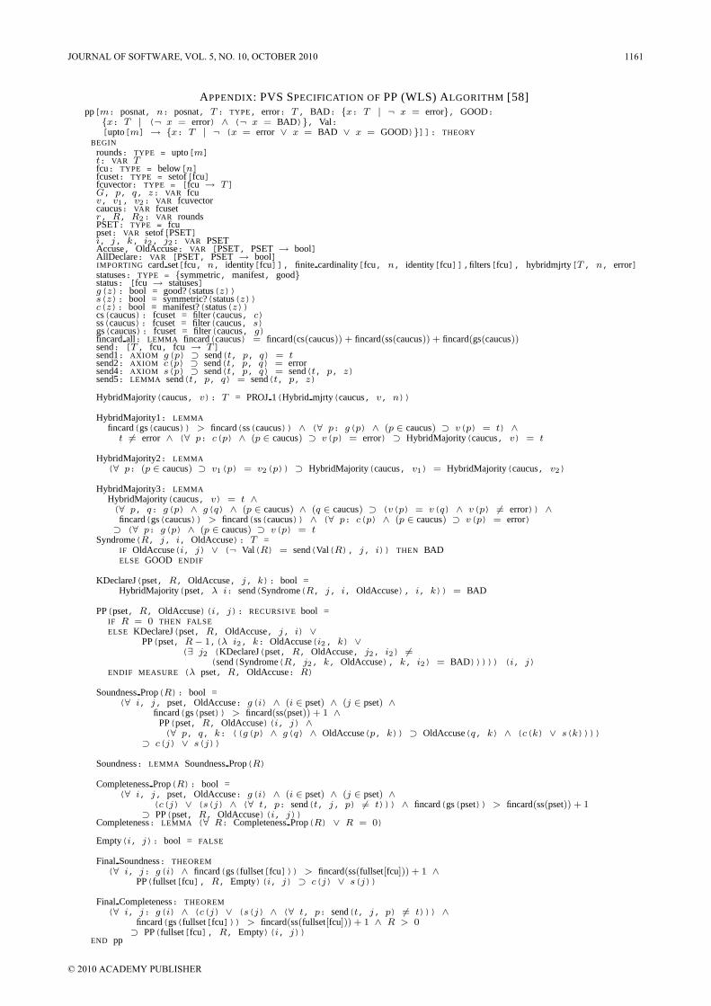
APPENDIX: PVS SPECIFICATION OF PP (WLS) ALGORITHM [58]pp[m: posnat, n: posnat, T: TYPE, error: T, BAD: x: T | ¬ x = error, GOOD:

x: T | (¬ x = error) ∧ (¬ x = BAD), Val:[upto[m] → x: T | ¬ (x = error ∨ x = BAD ∨ x = GOOD)]]: THEORY

BEGINrounds: TYPE = upto[m]t: VAR Tfcu: TYPE = below[n]fcuset: TYPE = setof[fcu]fcuvector: TYPE = [fcu → T]G, p, q, z: VAR fcuv, v1, v2: VAR fcuvectorcaucus: VAR fcusetr, R, R2: VAR roundsPSET: TYPE = fcupset: VAR setof[PSET]i, j, k, i2, j2: VAR PSETAccuse, OldAccuse: VAR [PSET, PSET → bool]AllDeclare: VAR [PSET, PSET → bool]IMPORTING card set[fcu, n, identity[fcu]], finite cardinality[fcu, n, identity[fcu]],filters[fcu], hybridmjrty[T, n, error]statuses: TYPE = symmetric, manifest, goodstatus: [fcu → statuses]g(z): bool = good?(status(z))s(z): bool = symmetric?(status(z))c(z): bool = manifest?(status(z))cs(caucus): fcuset = filter(caucus, c)ss(caucus): fcuset = filter(caucus, s)gs(caucus): fcuset = filter(caucus, g)fincard all: LEMMA fincard(caucus) = fincard(cs(caucus)) + fincard(ss(caucus)) + fincard(gs(caucus))send: [T, fcu, fcu → T]send1: AXIOM g(p) ⊃ send(t, p, q) = tsend2: AXIOM c(p) ⊃ send(t, p, q) = errorsend4: AXIOM s(p) ⊃ send(t, p, q) = send(t, p, z)send5: LEMMA send(t, p, q) = send(t, p, z)

HybridMajority(caucus, v): T = PROJ 1(Hybrid mjrty(caucus, v, n))

HybridMajority1: LEMMAfincard(gs(caucus)) > fincard(ss(caucus)) ∧ (∀ p: g(p) ∧ (p ∈ caucus) ⊃ v(p) = t) ∧

t = error ∧ (∀ p: c(p) ∧ (p ∈ caucus) ⊃ v(p) = error) ⊃ HybridMajority(caucus, v) = t

HybridMajority2: LEMMA(∀ p: (p ∈ caucus) ⊃ v1(p) = v2(p)) ⊃ HybridMajority(caucus, v1) = HybridMajority(caucus, v2)

HybridMajority3: LEMMAHybridMajority(caucus, v) = t ∧(∀ p, q: g(p) ∧ g(q) ∧ (p ∈ caucus) ∧ (q ∈ caucus) ⊃ (v(p) = v(q) ∧ v(p) = error)) ∧

fincard(gs(caucus)) > fincard(ss(caucus)) ∧ (∀ p: c(p) ∧ (p ∈ caucus) ⊃ v(p) = error)⊃ (∀ p: g(p) ∧ (p ∈ caucus) ⊃ v(p) = t

Syndrome(R, j, i, OldAccuse): T =IF OldAccuse(i, j) ∨ (¬ Val(R) = send(Val(R), j, i)) THEN BADELSE GOOD ENDIF

KDeclareJ(pset, R, OldAccuse, j, k): bool =HybridMajority(pset, λ i: send(Syndrome(R, j, i, OldAccuse), i, k)) = BAD

PP(pset, R, OldAccuse)(i, j): RECURSIVE bool =IF R = 0 THEN FALSEELSE KDeclareJ(pset, R, OldAccuse, j, i) ∨

PP(pset, R − 1,(λ i2, k: OldAccuse(i2, k) ∨(∃ j2 (KDeclareJ(pset, R, OldAccuse, j2, i2) =

(send(Syndrome(R, j2, k, OldAccuse), k, i2) = BAD))))) (i, j)ENDIF MEASURE (λ pset, R, OldAccuse: R)

Soundness Prop(R): bool =(∀ i, j, pset, OldAccuse: g(i) ∧ (i ∈ pset) ∧ (j ∈ pset) ∧

fincard(gs(pset)) > fincard(ss(pset)) + 1 ∧PP(pset, R, OldAccuse)(i, j) ∧(∀ p, q, k: ((g(p) ∧ g(q) ∧ OldAccuse(p, k)) ⊃ OldAccuse(q, k) ∧ (c(k) ∨ s(k))))

⊃ c(j) ∨ s(j))

Soundness: LEMMA Soundness Prop(R)

Completeness Prop(R): bool =(∀ i, j, pset, OldAccuse: g(i) ∧ (i ∈ pset) ∧ (j ∈ pset) ∧

(c(j) ∨ (s(j) ∧ (∀ t, p: send(t, j, p) = t))) ∧ fincard(gs(pset)) > fincard(ss(pset)) + 1⊃ PP(pset, R, OldAccuse)(i, j))

Completeness: LEMMA (∀ R: Completeness Prop(R) ∨ R = 0)

Empty(i, j): bool = FALSE

Final Soundness: THEOREM(∀ i, j: g(i) ∧ fincard(gs(fullset[fcu])) > fincard(ss(fullset[fcu])) + 1 ∧

PP(fullset[fcu], R, Empty)(i, j) ⊃ c(j) ∨ s(j))

Final Completeness: THEOREM(∀ i, j: g(i) ∧ (c(j) ∨ (s(j) ∧ (∀ t, p: send(t, j, p) = t))) ∧

fincard(gs(fullset[fcu])) > fincard(ss(fullset[fcu])) + 1 ∧ R > 0⊃ PP(fullset[fcu], R, Empty)(i, j))

END pp



The Use of AHP in Security Policy Decision Making: An Open Office Calc Application

Irfan Syamsuddin 1*

Department of Computer and Networking Engineering State Polytechnic of Ujung Pandang,

Makassar, Republic of Indonesia Email: [email protected]

Junseok Hwang

1 International IT Policy Program (ITPP), Technology Management, Economics and Policy Program (TEMEP),

Seoul National University, Seoul, Republic of Korea


Abstract— In this paper, we introduce a framework to guide decision makers evaluating information security policy performance. It is motivated by lack of adequate decision making mechanism with broader scopes and easy to use for the decision makers. The framework, which adopts Analytic hierarchy Process (AHP) methodology, is developed into a four level hierarchy (goal, criteria, sub-criteria, and alternatives) representing different aspects of information security policy. A survey based on AHP methodology was conducted to obtain decision maker preferences. Instead of relying on dedicated AHP software, we prefer to clearly demonstrate the process of AHP calculations by using Open Office Calc in data analysis. The aims are to show the applicability of open source software in handling AHP decision making problem and to help decision makers in understanding AHP data analysis procedures without relying on proprietary software. Results show that decision makers prefer availability of information security as highest priority, followed by confidentiality and integrity. The findings reflect future strategy in order to improve the effectiveness of information security policy in the organization. Index Terms—information security policy, decision making, Analytic Hierarchy Process, open source.

I. INTRODUCTION

The Analytical Hierarchy Process (AHP) is a decision

support system to deal with multi criteria decision making (MCDM) problems developed by Saaty [1]. It aims to quantify relative priorities for a given set of alternatives on a ratio scale, based on decision maker

judgments, by strictly following consistency standard of the pair wise comparison in the decision-making process.

Since a decision-maker bases judgments on knowledge and experience, then makes decisions accordingly, the AHP approach agrees well with the behavior of a decision maker. The strength of this approach is that it organizes tangible and intangible factors in a systematic way, and provides a structured yet relatively simple solution to the decision making problems [2]. In addition, by breaking a problem down in a logical fashion from the large, descending in gradual steps, to the smaller and smaller, one is able to connect, through simple paired comparison judgments, the small to the large. As a result, AHP has been widely adopted in various areas of research and practices these days such as government [18], business management [19] industry [20], health [21], education [22] and many other areas [4]. It mainly used for making selection, evaluation, cost and benefit analysis, resource allocations, planning and development, priority and ranking, and forecasting [23].

This study is proposed with the aim at filling the gap in information security policy literatures particularly from decision making perspectives. While the significance of implementing information security policy has been strongly recommended [7] not only at organizational levels [24] but even recently at national levels [25], there are only few studies on how a decision made with this regard [17].

Studies from academic [6] and professional [26] perspectives show lack of integrated decision making approaches in information security policy since they mostly focuses on technical [5,27] and managerial aspects of security such as ISO 17799, an international standard for information security management [28]. To understand the problem thoroughly, various aspects related to this domain should be studied and thus considered equally in decision making process.

On the grounds of the multi aspects nature of information security policy, we argue that this field is a

* Corresponding author: Irfan Syamsuddin Based on “Information Security Policy Decision Making: An AnalyticHierarchy Process Approach” by Junseok Hwang and Irfan Syamsuddinwhich appeared in The Proceedings of 3rd IEEE Asia InternationalConference on Modelling & Simulation AMS 2009 © IEEE.



kind of multi criteria decision making (MCDM) problem that can be overcome by using AHP method.

The primary focus of this study lies in the application of AHP through step by step mathematical calculation to solve decision making problem in the specific area of information security policy. Open Office Calc is selected to show details of AHP procedure and to demonstrate the potential of open source software as a powerful tool to solve multi criteria decision making problems.

The organization of this study is structured as follows. Section 2 presents literature review of information security. The next section presents our research objectives and methodology. Then, we introduce our AHP decision model in section 4. It is followed by analysis and discussion in the following. Finally, conclusion and future research direction are given in section 6.

II. LITERATURE REVIEW

Information security is defined as the set of laws, rules,

and practices that regulate how an organization manages, protects, and distributes resources to achieve specified security policy objectives [5]. These laws, rules, and practices must identify criteria for according individuals authority, and may specify conditions under which individuals are permitted to exercise their authority. To be meaningful, these laws, rules, and practices must provide individuals reasonable ability to determine whether their actions violate or comply with the policy [5, 6].

Among various information security and privacy controls, information security policy is considered as a soft approach to deal internally with security related issues to organizations [29]. It is intended to be main reference for organization to safely maintain data, information systems and general electronic base activities [6,29].

Basically, security policy determines technical security measures such as policies applied to firewall, virtual private network VPN and intranet/ internet communications. These policies determine what users may and may not do with respect to security and privacy countermeasures [27].

However, it is no longer the exclusive domain of technical issues [10] as mentioned by Ransbotham and Mitra [30] that many security breaches cases have shown information security has been more a management issue.

The role of information security policy is believed to be more important these days and has broader scope due to increasing cyber threats faced by many organizations [28]. Similarly, Bacik [7] argues that the impacts of information security breaches have been increasingly affecting non technical aspect of organizations such as organizational human resources, finance and stock market. Thus, due to such changes there is strong requirement to reevaluate ISP performance by kindly considering all of related aspects.

In order to accommodate different perspectives found in literature, we propose a classification based on main information security policy aspects as mentioned below.

• Aspect of Management. Information security management with standardized security policy is confirmed to become a required tool by many organizations particularly those that rely heavily on the Internet to conduct their operations [8]. Compliance to international standard such as ISO 17799 [28], and implementation of data classification procedures and access control [31] are few examples of emphasis in managing information security. This can be done properly with strong support from top management combined with a commitment by all members of the organization to explicitly prevent the possibility of security risks [9].

• Aspect of Technology. Technical side of information security in terms of data, hardware, and applications has become a concern since the beginning of the computer era. This includes terminal security, network security, and Internet security [10]. The significance of technical aspect of information security can be seen from ongoing research in this area such as virus [32], worm [33] and other technical countermeasures [10] from personal computer to the Internet. In short, various security technologies at all levels are still believed as the key elements to combat information security attacks [10].

• Aspect of Economy. In [11], Anderson introduces a new economic perspective of information security. Based on his work, the economic of information security has gained a great intention from researchers academic and professional, such as cost and benefits analysis [34] and security investment evaluation [12] to deal with growing information security issues. Filipek [8] affirms that information security has been a serious business priority since many evidences show how cyber attacks have damaged business reputation of many companies in stock market [13].

• Aspect of Culture. Compare to previous aspects, information security culture is one that lately received serious attention by practitioners and academies. Lack of inherent security awareness culture was believed as the main source of internal security breaches in some organization [14]. Survey shows a significant amount of cyber security breaches come from internal organization [35]. Schlienger and Teufel [16] justify that information security policy will be effective only if adequate security culture exist within an organization [16]. There are many ways to establish security culture. While Herath and Tao [29] confirm the role of penalties and pressures in establishing security culture, other researchers argue that security education [15] and organizational leadership [9] are paramount.



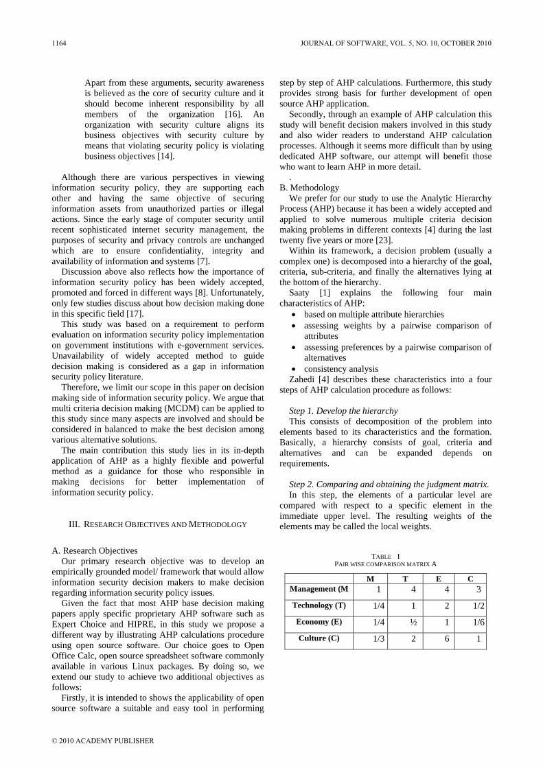
Apart from these arguments, security awareness is believed as the core of security culture and it should become inherent responsibility by all members of the organization [16]. An organization with security culture aligns its business objectives with security culture by means that violating security policy is violating business objectives [14].

Although there are various perspectives in viewing

information security policy, they are supporting each other and having the same objective of securing information assets from unauthorized parties or illegal actions. Since the early stage of computer security until recent sophisticated internet security management, the purposes of security and privacy controls are unchanged which are to ensure confidentiality, integrity and availability of information and systems [7].

Discussion above also reflects how the importance of information security policy has been widely accepted, promoted and forced in different ways [8]. Unfortunately, only few studies discuss about how decision making done in this specific field [17].

This study was based on a requirement to perform evaluation on information security policy implementation on government institutions with e-government services. Unavailability of widely accepted method to guide decision making is considered as a gap in information security policy literature.

Therefore, we limit our scope in this paper on decision making side of information security policy. We argue that multi criteria decision making (MCDM) can be applied to this study since many aspects are involved and should be considered in balanced to make the best decision among various alternative solutions.

The main contribution this study lies in its in-depth application of AHP as a highly flexible and powerful method as a guidance for those who responsible in making decisions for better implementation of information security policy.

III. RESEARCH OBJECTIVES AND METHODOLOGY

A. Research Objectives

Our primary research objective was to develop an empirically grounded model/ framework that would allow information security decision makers to make decision regarding information security policy issues.

Given the fact that most AHP base decision making papers apply specific proprietary AHP software such as Expert Choice and HIPRE, in this study we propose a different way by illustrating AHP calculations procedure using open source software. Our choice goes to Open Office Calc, open source spreadsheet software commonly available in various Linux packages. By doing so, we extend our study to achieve two additional objectives as follows:

Firstly, it is intended to shows the applicability of open source software a suitable and easy tool in performing

step by step of AHP calculations. Furthermore, this study provides strong basis for further development of open source AHP application.

Secondly, through an example of AHP calculation this study will benefit decision makers involved in this study and also wider readers to understand AHP calculation processes. Although it seems more difficult than by using dedicated AHP software, our attempt will benefit those who want to learn AHP in more detail.

. B. Methodology

We prefer for our study to use the Analytic Hierarchy Process (AHP) because it has been a widely accepted and applied to solve numerous multiple criteria decision making problems in different contexts [4] during the last twenty five years or more [23].

Within its framework, a decision problem (usually a complex one) is decomposed into a hierarchy of the goal, criteria, sub-criteria, and finally the alternatives lying at the bottom of the hierarchy.

Saaty [1] explains the following four main characteristics of AHP:

• based on multiple attribute hierarchies • assessing weights by a pairwise comparison of

attributes • assessing preferences by a pairwise comparison of

alternatives • consistency analysis

Zahedi [4] describes these characteristics into a four steps of AHP calculation procedure as follows:

Step 1. Develop the hierarchy This consists of decomposition of the problem into

elements based to its characteristics and the formation. Basically, a hierarchy consists of goal, criteria and alternatives and can be expanded depends on requirements.

Step 2. Comparing and obtaining the judgment matrix. In this step, the elements of a particular level are

compared with respect to a specific element in the immediate upper level. The resulting weights of the elements may be called the local weights.

TABLE I PAIR WISE COMPARISON MATRIX A

M T E C Management (M 1 4 4 3

Technology (T) 1/4 1 2 1/2

Economy (E) 1/4 ½ 1 1/6

Culture (C) 1/3 2 6 1



The matrix A can be defined by

⎥⎥⎥⎥

⎦

⎤

⎢⎢⎢⎢

⎣

⎡

=

nnnn

n

n

aaa

aaaaaa

A

21

22221

11211

,

where n is the order of matrix. Then the consistency property in the pair wise

comparison is examined by a two steps procedure as follows [1]:

• Develop the normalized pariwise comparison matrix

A1

⎥⎥⎥⎥

⎦

⎤

⎢⎢⎢⎢

⎣

⎡

=

nnnn

n

n

aaa

aaaaaa

A

'''

''''''

21

22221

11211

1

and

∑=

= n

iij

ijij

a

aa

1

for i , j = 1, 2,…, n.

• Test the consistency property. Where CI is the consistency index, CR is the

consistency ratio, λmax is the largest eigenvalue of the pair wise comparison matrix, n is the matrix order, and RI is random index. Table 3 shows a set of recommended RI values presented by Saaty [1].

TABLE II RANDOM INDEX

N 1 2 3 4 5

RI 0 0 0.52 0.89 1.11

N 6 7 8 9 10

RI 1.25 1.35 1.40 1.45 1.49

This is argued as one of AHP’s advantages which able

to measure whether or not inconsistency occurs in the judgment process. If CR values are > 0.10 for a matrix larger than 4x4, it indicates an inconsistent judgment. In some parts decision makers should revise the original values in the pair wise comparison matrix until desired consistency level reached.

Step 3: Local weights and consistency of comparisons. In this step, local weights of the elements are

calculated from the judgment matrices using the eigenvector method (EVM). The normalized eigenvector corresponding to the principal eigenvalue of the judgment matrix provides the weights of the corresponding elements.

⎥⎥⎥⎥

⎦

⎤

⎢⎢⎢⎢

⎣

⎡

=

nw

ww

W 2

1

, and n

aw

n

iij

i

∑== 1

' for i = 1, 2,…, n

Then W’ is obtained as a new matrix based on

multiplication between matrix A and W as described below

⎥⎥⎥⎥

⎦

⎤

⎢⎢⎢⎢

⎣

⎡

==

nw

ww

WAW

'

''

.' 2

1

and ⎟⎟⎠

⎞⎜⎜⎝

⎛+++=

n

n

ww

ww

ww

n'''1

2

2

1

1maxλ

Where W’ is the eigenvector, wi is the eigenvalue of

criterion I, and λmax is the largest eigenvalue of the pair wise comparison matrix.

Step 4: Aggregation of weights across various levels to

obtain the final weights of alternatives. This final step of AHP procedure where the local

weights of elements of different levels are aggregated to obtain final weights of the decision alternatives (elements at the lowest level).

IV. AHP DECISION MODEL

In this section, the development of AHP decision

model for information securoty policy is explained. We construct the hierarchy for information security policy decision making that combines multi criteria, different aspects and alternatives. It adopts AHP which enables structuring, measurement and synthesizing of decision hierarchy [1] to make good decisions.

Figure 1 shows the structure of our AHP decision model. It is a four layer hierarchy consists of goal, criteria, sub-criteria and alternatives. All layers are described as follows.



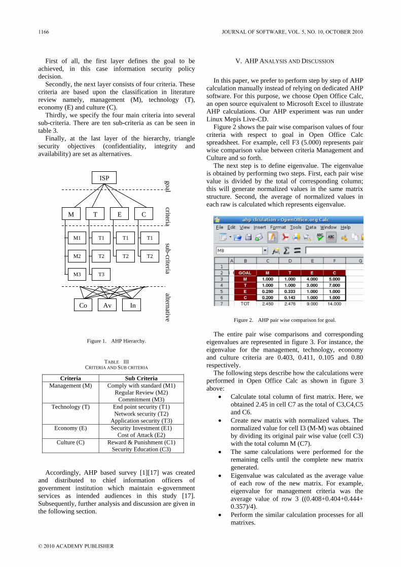
First of all, the first layer defines the goal to be achieved, in this case information security policy decision.

Secondly, the next layer consists of four criteria. These criteria are based upon the classification in literature review namely, management (M), technology (T), economy (E) and culture (C).

Thirdly, we specify the four main criteria into several sub-criteria. There are ten sub-criteria as can be seen in table 3.

Finally, at the last layer of the hierarchy, triangle security objectives (confidentiality, integrity and availability) are set as alternatives.

Figure 1. AHP Hierarchy.

TABLE III CRITERIA AND SUB CRITERIA

Criteria Sub Criteria Management (M) Comply with standard (M1)

Regular Review (M2) Commitment (M3)

Technology (T) End point security (T1) Network security (T2)

Application security (T3) Economy (E) Security Investment (E1)

Cost of Attack (E2) Culture (C) Reward & Punishment (C1)

Security Education (C3)

Accordingly, AHP based survey [1][17] was created

and distributed to chief information officers of government institution which maintain e-government services as intended audiences in this study [17]. Subsequently, further analysis and discussion are given in the following section.

V. AHP ANALYSIS AND DISCUSSION

In this paper, we prefer to perform step by step of AHP

calculation manually instead of relying on dedicated AHP software. For this purpose, we choose Open Office Calc, an open source equivalent to Microsoft Excel to illustrate AHP calculations. Our AHP experiment was run under Linux Mepis Live-CD.

Figure 2 shows the pair wise comparison values of four criteria with respect to goal in Open Office Calc spreadsheet. For example, cell F3 (5.000) represents pair wise comparison value between criteria Management and Culture and so forth.

The next step is to define eigenvalue. The eigenvalue is obtained by performing two steps. First, each pair wise value is divided by the total of corresponding column; this will generate normalized values in the same matrix structure. Second, the average of normalized values in each raw is calculated which represents eigenvalue.

Figure 2. AHP pair wise comparison for goal.

The entire pair wise comparisons and corresponding eigenvalues are represented in figure 3. For instance, the eigenvalue for the management, technology, economy and culture criteria are 0.403, 0.411, 0.105 and 0.80 respectively.

The following steps describe how the calculations were performed in Open Office Calc as shown in figure 3 above:

• Calculate total column of first matrix. Here, we obtained 2.45 in cell C7 as the total of C3,C4,C5 and C6.

• Create new matrix with normalized values. The normalized value for cell I3 (M-M) was obtained by dividing its original pair wise value (cell C3) with the total column M (C7).

• The same calculations were performed for the remaining cells until the complete new matrix generated.

• Eigenvalue was calculated as the average value of each row of the new matrix. For example, eigenvalue for management criteria was the average value of row 3 ((0.408+0.404+0.444+ 0.357)/4).

• Perform the similar calculation processes for all matrixes.

M

ISP

T

M1

E C

M2

M3

T1

T2

T3

T1

T2

T1

T2

Co Av In

goal criteria

sub-criteria alternative



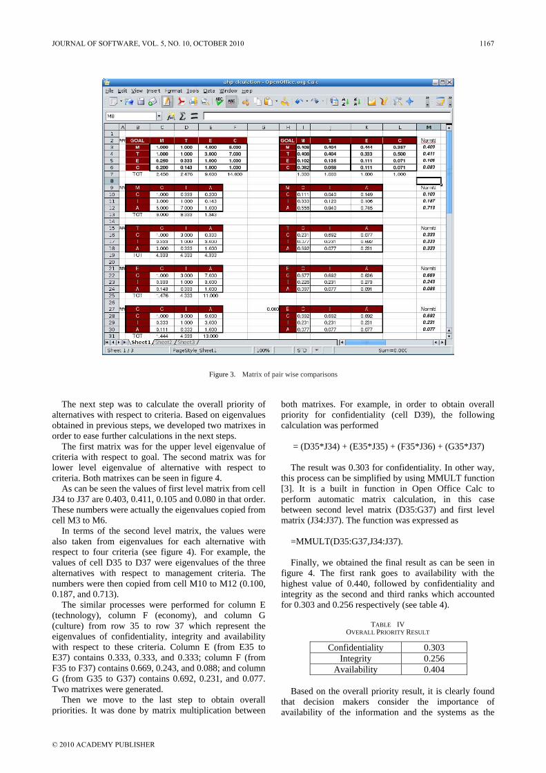
Figure 3. Matrix of pair wise comparisons

The next step was to calculate the overall priority of

alternatives with respect to criteria. Based on eigenvalues obtained in previous steps, we developed two matrixes in order to ease further calculations in the next steps.

The first matrix was for the upper level eigenvalue of criteria with respect to goal. The second matrix was for lower level eigenvalue of alternative with respect to criteria. Both matrixes can be seen in figure 4.

As can be seen the values of first level matrix from cell J34 to J37 are 0.403, 0.411, 0.105 and 0.080 in that order. These numbers were actually the eigenvalues copied from cell M3 to M6.

In terms of the second level matrix, the values were also taken from eigenvalues for each alternative with respect to four criteria (see figure 4). For example, the values of cell D35 to D37 were eigenvalues of the three alternatives with respect to management criteria. The numbers were then copied from cell M10 to M12 (0.100, 0.187, and 0.713).

The similar processes were performed for column E (technology), column F (economy), and column G (culture) from row 35 to row 37 which represent the eigenvalues of confidentiality, integrity and availability with respect to these criteria. Column E (from E35 to E37) contains 0.333, 0.333, and 0.333; column F (from F35 to F37) contains 0.669, 0.243, and 0.088; and column G (from G35 to G37) contains 0.692, 0.231, and 0.077. Two matrixes were generated.

Then we move to the last step to obtain overall priorities. It was done by matrix multiplication between

both matrixes. For example, in order to obtain overall priority for confidentiality (cell D39), the following calculation was performed

= (D35*J34) + (E35*J35) + (F35*J36) + (G35*J37) The result was 0.303 for confidentiality. In other way,

this process can be simplified by using MMULT function [3]. It is a built in function in Open Office Calc to perform automatic matrix calculation, in this case between second level matrix (D35:G37) and first level matrix (J34:J37). The function was expressed as

=MMULT(D35:G37,J34:J37). Finally, we obtained the final result as can be seen in

figure 4. The first rank goes to availability with the highest value of 0.440, followed by confidentiality and integrity as the second and third ranks which accounted for 0.303 and 0.256 respectively (see table 4).

TABLE IV OVERALL PRIORITY RESULT

Confidentiality 0.303 Integrity 0.256

Availability 0.404 Based on the overall priority result, it is clearly found

that decision makers consider the importance of availability of the information and the systems as the



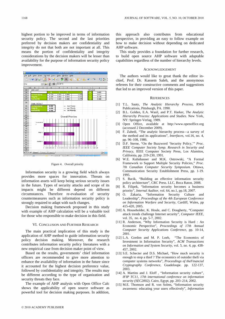
highest portion to be improved in terms of information security policy. The second and the last priorities preferred by decision makers are confidentiality and integrity do not that both are not important at all. This means the portion of confidentiality and integrity considerations by the decision makers will be lesser than availability for the purpose of information security policy improvement.

Figure 4. Overall priority

Information security is a growing field which always provides more spaces for innovation. Threats on information assets will keep being serious security issues in the future. Types of security attacks and scope of its impacts might be different depend on different circumstances. Therefore re-evaluation of security countermeasures such as information security policy is strongly required to adapt with such changes.

Decision making framework proposed in this study with example of AHP calculation will be a valuable tool for those who responsible to make decision in this field.

VI. CONCLUSION AND FURTHER RESEARCH

The main practical implication of this study is the application of AHP method to guide information security policy decision making. Moreover, the research contributes information security policy literatures with a new empirical case from decision maker point of view.

Based on the results, governments’ chief information officers are recommended to give more attention to enhance the availability of information in the future since it accounted for the highest decision preference value, followed by confidentiality and integrity. The results may be different according to the type of organization and security threats they face.

The example of AHP analysis with Open Office Calc shows the applicability of open source software as powerful tool for decision making purposes. In addition,

this approach also contributes from educational perspective, in providing an easy to follow example on how to make decision without depending on dedicated AHP software.

This study provides a foundation for further research, to build open source AHP software with adaptable capabilities regardless of the number of hierarchy levels.

ACKNOWLEDGEMENT

The authors would like to great thank the editor in-chief, Prof. Dr. Kassem Saleh, and the anonymous referees for their constructive comments and suggestions that led to an improved version of this paper.

REFERENCES

[1] T.L. Saaty, The Analytic Hierarchy Process, RWS Publications, Pittsburgh, PA. 1990.

[2] B.L. Golden, E.A. Wasil, and P.T. Harker, The Analytic Hierarchy Process: Applications and Studies. New York, NY: Springer-Verlag, 1989.

[3] Open Office, available at http://www.openoffice.org (accessed 2 December 2009).

[4] F. Zahedi, “The analytic hierarchy process—a survey of the method and its applications”, Interfaces, vol.16, no. 4, pp. 96–108, 1986.

[5] D.F. Sterne, “On the Buzzword ‘Security Policy,’” Proc. IEEE Computer Society Symp. Research in Security and Privacy, IEEE Computer Society Press, Los Alamitos, California, pp. 219-230, 1991.

[6] W.E. Kuhnhauser and M.K. Ostrowski, “A Formal Framework to Support Multiple Security Policies,” Proc. 7th Canadian Computer Security Symposium. Ottawa, Communication Security Establishment Press, pp. 1-19. 1995.

[7] S. Bacik, “Building an effective information security policy architecture”, CRC Press. LLC, Boca Raton, 2008.

[8] R. Filipek, “Information security becomes a business priority”, Internal Auditor, vol. 64, no.1, pp.18, 2007.

[9] O. Zakaria, “Information Security Culture and Leadership”, Proceedings of the 4th European Conference on Information Warfare and Security, Cardiff, Wales, pp 415-420, 2005.

[10] A. Householder, K. Houle, and C. Dougherty, “Computer attack trends challenge Internet security”, Computer IEEE, vol. 35, no. 4, pp. 5-7, 2002.

[11] R. Anderson, “Why Information Security is Hard : An Economic Perspective”, Proceedings of 17th Annual Computer Security Applications Conference, pp. 10-14, 2001.

[12] L.A. Gordon and M. P. Loeb, “The Economics of Investment in Information Security”, ACM Transactions on Information and System Security, vol. 5, no. 4, pp. 438-457, 2002.

[13] S.E. Schecter and D.S. Michael, “How much security is enough to stop a thief ? The economics of outsider theft via computer systems networks”, Proceedings of theFinancial Cryptography Conference, Guadeloupe. pp. 122-137, 2003.

[14] A. Martins and J. Eloff , “Information security culture”, IFIP TC11, 17th international conference on information security (SEC2002), Cairo, Egypt, pp. 203–214, 2002.

[15] M.E. Thomson and R. von Solms, “Information security awareness: educating your users effectively”, Information



Management and Computer Security, vol. 6, no. 4, pp. 167–173, 1998.

[16] T. Schlienger and S. Teufel, “Information Security Culture: The Socio-Cultural Dimension in Information Security Management”, Proceedings of the IFIP TC11 17th International Conference on Information Security, pp. 191 – 202, 2002.

[17] J. Hwang and I. Syamsuddin, “Information Security Policy Decision Making: An Analytic Hierarchy Process Approach”, Proceeding of IEEE 2009 Third Asia International Conference on Modelling & Simulation, pp. 158-163, 2009.

[18] Kahraman, Cengiz, Demirel, N. Cetin, Demirel and Tufan, “Prioritization of e-Government strategies using a SWOT-AHP analysis: the case of Turkey”, European Journal of Information Systems, vol. 16, no. 3, pp. 284-298, 2007.

[19] M.C. Lin, C.C. Wang, M.S. Chen and C.A. Chang, Using AHP and TOPSIS approaches in customer-driven product design process, Computers in Industry , vol. 59, no. 1, pp. 17–31, 2008.

[20] C.Unal and G.G. Mucella, “Selection of ERP suppliers using AHP tools in the clothing industry”, International Journal of Clothing Science and Technology, vol. 21, no. 4, pp. 239-251, 2009.

[21] L.A. Vidal, E. Sahin, N. Martelli, M. Berhoune and B. Bonan, “Applying AHP to select drugs to be produced by anticipation in a chemotherapy compounding unit”, Expert Systems with Applications, vol. 37, no. 2, pp. 1528-1534, 2010.

[22] W. Ho, H.E. Higson, P.K. Dey, X. Xu and R. Bahsoon, “Measuring performance of virtual learning environment system in higher education”, Quality Assurance in Education , vol.17, no. 1, pp. 6-29, 2009.

[23] O.S. Vaidya and S. Kumar, “Analytic hierarchy process: An overview of applications”, European Journal of Operational Research, vol. 169, no. 1, pp. 1–29, 2006.

[24] H. Fulford and N.F.Doherty, “The application of information security policies in large UK-based organizations: an exploratory investigation”, Information Management & Computer Security, vol. 11, no. 3, pp. 106 – 114, 2003.

[25] C.Y. Ku, Y.W. Chang and D.C. Yen, “National information security policy and its implementation: A case study in Taiwan”, Telecommunications Policy, vol. 33 , no. 7, pp. 371-384, 2009.

[26] K. Shannon, P. Anne, H. Ben, P. Chad and C. Matt, “Information security threats and practices in small businesses”, Information Systems Management, vol. 22, no 2 pp. 7-19, 2005.

[27] A.Herzog and N. Shahmehri, “Usable Set-up of Runtime Security Policies”, Information Management & Computer Security, vol. 15, no. 5, pp 394-407, 2007.

[28] M.C. Lee and T. Chang, “Applying ISO 17799:2005 in information security management”, International Journal

of Services and Standards, vol. 3, no. 3, pp.352 – 373, 2007.

[29] T. Herath and H.R. Rao, “Encouraging information security behaviors in organizations: Role of penalties, pressures and perceived effectiveness”, Decision Support Systems, vol. 47, no. 2, pp. 154-165, 2009.

[30] S. Ransbotham and S. Mitra, “Choice and Chance: A Conceptual Model of Paths to Information Security Compromise”, Information Systems Research, vol. 20, no. 1, pp. 121-139, 2009.

[31] C. Huang, J. Sun, X. Wang and Y.J. Si, “Security Policy Management for Systems Employing Role Based Access Control Model”, Information Technology Journal, vol. 8, no. 5, pp. 726-734, 2009.

[32] C. Jin, J. Liu, and Q. Deng, “Network Virus Propagation Model Based on Effects of Removing Time and User Vigilance”, International Journal of Network Security, vol. 9, no. 2, pp. 156-163, 2009.

[33] T. Komninos, P. Spirakis, Y.C. Stamatiou, G. Vavitsas, “A Worm Propagation Model based on Scale Free Network Structures and People's Email Acquaintance Profiles”, International Journal of Computer Science and Network Security, vol. 7, no. 2, pp. 308-315, 2007.

[34] S.A. Butler, “Security attribute evaluation method: a cost-benefit approach”, Proceedings of the 24th International Conference on Software Engineering, pp. 232-240, 2002.

[35] Verizon, “Data Breach Investigations Report 2009”, available at: http://www.verizonbusiness.com (accessed 22 February 2010).

Irfan Syamsuddin is a lecturer at State Polytechnic of

Ujung Pandang, Makassar, Indonesia. Currently he is pursuing PhD research at International Information Technology Policy Program (ITPP), Seoul National University Republic of Korea. Previously, he obtained B.Eng degree in Electrical Engineering from Hasanuddin University, Indonesia, then received his Postgraduate Diploma in Business Electronic Commerce and Master of Commerce in Internet Security Management degrees both from Curtin University of Technology, Perth, Australia.

Prof. Junseok Hwang is a US-trained Engineer and

currently serving as a Director and Dean of the Technology Management, Economics and Policy Program (TEMEP) and of the International Information Technology Policy Program (ITPP) at the Seoul National University and Associate Professor at the Seoul National University Republic of Korea.Dr. Hwang received his B.S. degree from Yonsei University, Korea specializing in Mathematics, his M.S. degree in Telecommunications from the Univ. of Colorado, and his Ph.D. in Information Science and Telecommunications from the University of Pittsburgh, Pittsburgh, PA in the United States.



Adaptive Multi-agent System: Cooperation and Structures Emergence

Imane BOUSSEBOUGH1, Ramdane MAAMRI2, Zaïdi SAHNOUN3

Laboratory LIRE Department of Computer Science Faculty of Science of the engineer

University Mentouri of Constantine. 25000. Algeria

Email: 1 [email protected], 2 [email protected] , 3 [email protected] Abstract—Nowadays, development of adaptive multi-agent systems has attracted recent attention. Adaptive systems are capable of adapting themselves to unforeseen changes of their environment in autonomous manner. We are interested, in this paper, to adaptation in cooperative systems where agents share a same goal. We propose an adaptive approach based on interaction evaluation and genetic algorithms. Agents, in this approach, have the ability to reorganize themselves in order to bring closer agents capable of cooperating in problem solving. The adaptation task is accomplished at both local and global levels. We present here details of this approach and we show some preliminary experimentation results. Index Terms—adaptation, multi-agent, genetic algorithm, cooperation, interaction evaluation

I. INTRODUCTION

Multi-agent systems can be seen as societies of interacting agents. Interaction allows agents to find each other and then to exchange information. In such systems, each agent is capable of some useful activities, but being plunged in an artificial society communicating and cooperating with others it is able to enhance its performance and the society’s one. Thus, the main issues and the foundations of distributed artificial intelligence are the organisation, coordination and cooperation [21].

However, applications are becoming more and more open and complex such as e-learning, information retrieving and filtering, market place, e-commerce, e-business. Development of adaptive multi-agent systems, to deal with this complexity, has attracted recent attention. Adaptive multi-agent systems must be capable to adapt themselves to unforeseen situations in an autonomous manner. An adaptive system is one in which the structure is capable of changing dynamically [12], [1], [7].

We are interested, in this paper, to cooperative multi-agent systems immersed in dynamic environment. We propose an adaptive approach based on interaction evaluation and genetic algorithms. The system, in our approach, is composed of a set of Task Agents (TAi) that must fulfil the system function and a Mediator Agent responsible of reorganizing the system if this last is in

disturbances. The system adapts itself in order to have a cooperative organizational structure; it means that the good agent will be at the good place. For that, task agents have cooperative beliefs about each other; perceive system’s disturbances (at local level) from their interactions with each other, then correct cooperative beliefs and, if necessary, send disturbance signal to Mediator Agent. This last is responsible of reorganizing the system when it is judged in disturbances (at global level); the Mediator Agent uses genetic algorithm to enhance system cooperation.

We present in the section 2 problematic of adaptation in our approach, section 3 presents our approach of adaptive system GAMuS, section 4 shows experimentation and preliminary results and finally we give conclusion and perspectives.

II. PROBLEMATIC

Multi-agent systems have become popular over the last few years for building complex and adaptive software systems. Such systems should have the capability of dynamically adapting themselves according to environment changes, they must be capable of: • identifying circumstances that require adaptation, • and accordingly improve their performance in an

autonomous manner [8]. Adaptation can take different forms such as change of

structure, of content, of relations, of localization of programs or data; and can be at local level or at global one.

We believe that, in adaptive multi-agent systems, adaptability must be a characteristic of agents themselves, they must be able to perceive unforeseen changes of the environment, and act in consequence. In multi agent systems, adaptation can be closely related to evolution of the system structure [3]. At the other hand, to solve complex problems, agents must work cooperatively with other agents in a heterogeneous environment.

Moreover, genetic approach, can harness the power of natural selection to produce communities of agents well suited to their niches, even in environments that are too complex or dynamic for detailed human analysis. In a genetic based system, solutions emerge from a continuous process of adaptive engagement with the



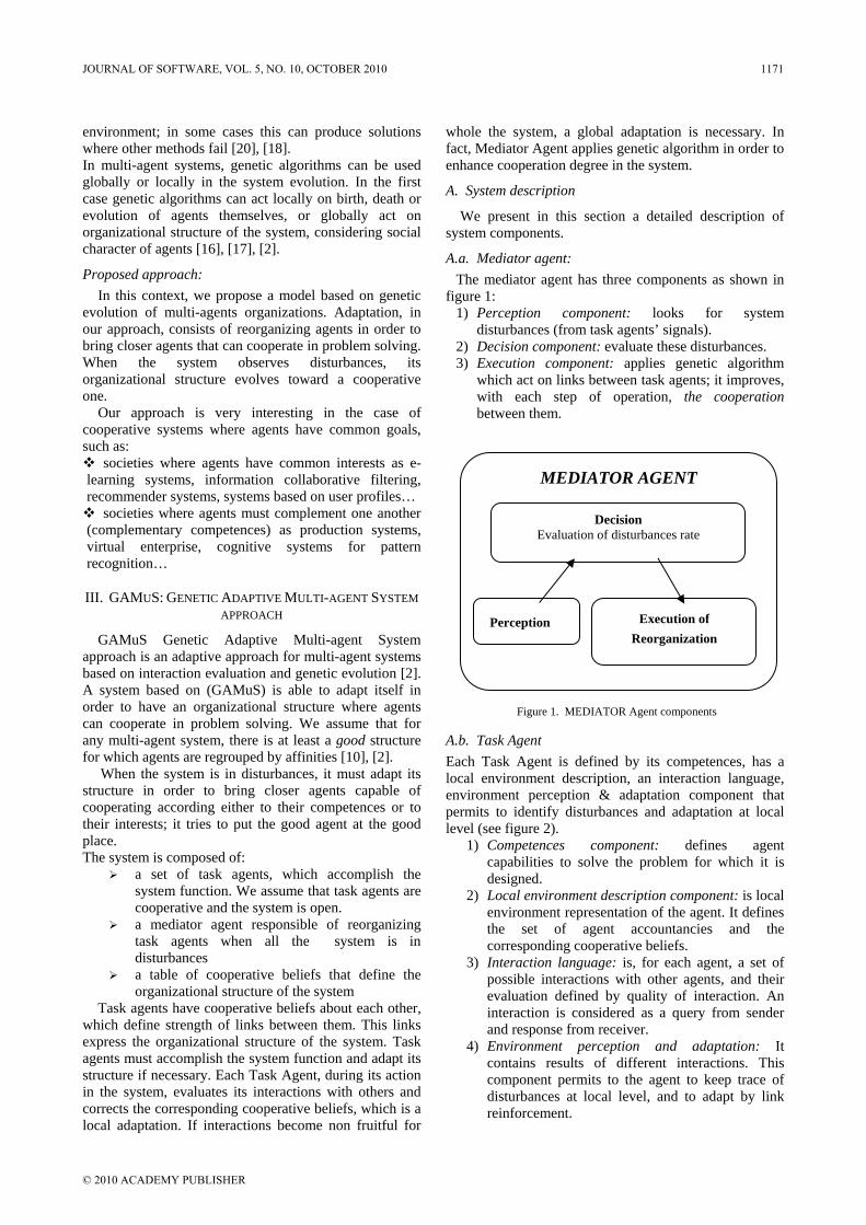
environment; in some cases this can produce solutions where other methods fail [20], [18]. In multi-agent systems, genetic algorithms can be used globally or locally in the system evolution. In the first case genetic algorithms can act locally on birth, death or evolution of agents themselves, or globally act on organizational structure of the system, considering social character of agents [16], [17], [2].

Proposed approach: In this context, we propose a model based on genetic

evolution of multi-agents organizations. Adaptation, in our approach, consists of reorganizing agents in order to bring closer agents that can cooperate in problem solving. When the system observes disturbances, its organizational structure evolves toward a cooperative one.

Our approach is very interesting in the case of cooperative systems where agents have common goals, such as:

societies where agents have common interests as e-learning systems, information collaborative filtering, recommender systems, systems based on user profiles…

societies where agents must complement one another (complementary competences) as production systems, virtual enterprise, cognitive systems for pattern recognition…

III. GAMUS: GENETIC ADAPTIVE MULTI-AGENT SYSTEM APPROACH

GAMuS Genetic Adaptive Multi-agent System approach is an adaptive approach for multi-agent systems based on interaction evaluation and genetic evolution [2]. A system based on (GAMuS) is able to adapt itself in order to have an organizational structure where agents can cooperate in problem solving. We assume that for any multi-agent system, there is at least a good structure for which agents are regrouped by affinities [10], [2].

When the system is in disturbances, it must adapt its structure in order to bring closer agents capable of cooperating according either to their competences or to their interests; it tries to put the good agent at the good place. The system is composed of:

a set of task agents, which accomplish the system function. We assume that task agents are cooperative and the system is open.

a mediator agent responsible of reorganizing task agents when all the system is in disturbances

a table of cooperative beliefs that define the organizational structure of the system

Task agents have cooperative beliefs about each other, which define strength of links between them. This links express the organizational structure of the system. Task agents must accomplish the system function and adapt its structure if necessary. Each Task Agent, during its action in the system, evaluates its interactions with others and corrects the corresponding cooperative beliefs, which is a local adaptation. If interactions become non fruitful for

whole the system, a global adaptation is necessary. In fact, Mediator Agent applies genetic algorithm in order to enhance cooperation degree in the system.

A. System description

We present in this section a detailed description of system components.

A.a. Mediator agent: The mediator agent has three components as shown in

figure 1: 1) Perception component: looks for system

disturbances (from task agents’ signals). 2) Decision component: evaluate these disturbances. 3) Execution component: applies genetic algorithm

which act on links between task agents; it improves, with each step of operation, the cooperation between them.

A.b. Task Agent Each Task Agent is defined by its competences, has a local environment description, an interaction language, environment perception & adaptation component that permits to identify disturbances and adaptation at local level (see figure 2).

1) Competences component: defines agent capabilities to solve the problem for which it is designed.

2) Local environment description component: is local environment representation of the agent. It defines the set of agent accountancies and the corresponding cooperative beliefs.

3) Interaction language: is, for each agent, a set of possible interactions with other agents, and their evaluation defined by quality of interaction. An interaction is considered as a query from sender and response from receiver.

4) Environment perception and adaptation: It contains results of different interactions. This component permits to the agent to keep trace of disturbances at local level, and to adapt by link reinforcement.

MEDIATOR AGENT

Decision Evaluation of disturbances rate

Perception Execution of Reorganization

Figure 1. MEDIATOR Agent components



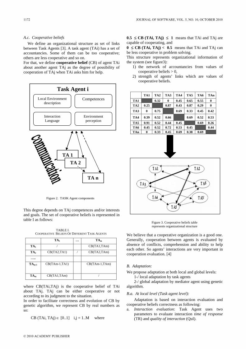
A.c. Cooperative beliefs We define an organizational structure as set of links

between Task Agents [3]. A task agent (TAi) has a set of accountancies. Some of them can be too cooperative; others are less cooperative and so on. For that, we define cooperative belief (CB) of agent TAi about another agent TAj as the degree of possibility of cooperation of TAj when TAi asks him for help.

This degree depends on TAj competences and/or interests and goals. The set of cooperative beliefs is represented in table I as follows: where CB(TAi,TAj) is the cooperative belief of TAi about TAj. TAj can be either cooperative or not according to its judgment to the situation. In order to facilitate correctness and evolution of CB by genetic algorithm, we represent CB by real numbers as so:

CB (TAi, TAj) ∈ [0..1] i,j = 1..M where

0.5 ≤ CB (TAi, TAj) ≤ 1 means that TAi and TAj are capable of cooperating, and 0 ≤ CB (TAi, TAj) < 0.5 means that TAi and TAj can be less cooperative in problem solving. This structure represents organizational information of the system (see figure3):

1) the network of accountancies from values of cooperative beliefs > 0,

2) strength of agents’ links which are values of cooperative beliefs.

We believe that a cooperative organization is a good one. Generally, cooperation between agents is evaluated by absence of conflicts, comprehension and ability to help each other. So agents’ interactions are very important in cooperation evaluation. [4]

B. Adaptation: We propose adaptation at both local and global levels:

1-/ local adaptation by task agents 2-/ global adaptation by mediator agent using genetic

algorithm.

B.a. At local level (Task agent level): Adaptation is based on interaction evaluation and

cooperative beliefs correctness as following: a. Interaction evaluation: Task Agent uses two

parameters to evaluate interaction time of response (TR) and quality of interaction (QuI).

Figure 3. Cooperative beliefs table represents organizational structure

TA1 TA2 TA3 TA4 TA5 TA6 TAn

TA1 0.32 0 0.45 0.65 0.55 0 TA2 0.25 0.87 0.43 0.87 0.29 0

TA3 0 0.75 0.69 0.33 0.45 0.42

TA4 0.39 0.52 0.66 0.69 0.52 0.53

TA5 0.91 0.52 0.44 0.45 0.69 0.26 TA6 0.45 0.52 0.72 0.53 0.45 0.44 TAn 0 0.33 0.45 0.69 0.38 0.69

TABLE I. COOPERATIVE BELIEFS OF DIFFERENT TASK AGENTS

TA1 … TAm

TA1 / CB(TA1,TAm)

TA2 CB(TA2,TA1) / CB(TA2,TAm)

…..

TAm-1 CB(TAm-1,TA1) CB(TAm-1,TAm)

TAm CB(TA1,TAm) /

TA 1 TA 2

TA n

Task Agent i Competences

Environment perception

Interaction Language

Local Environment description

Figure 2. TASK Agent components



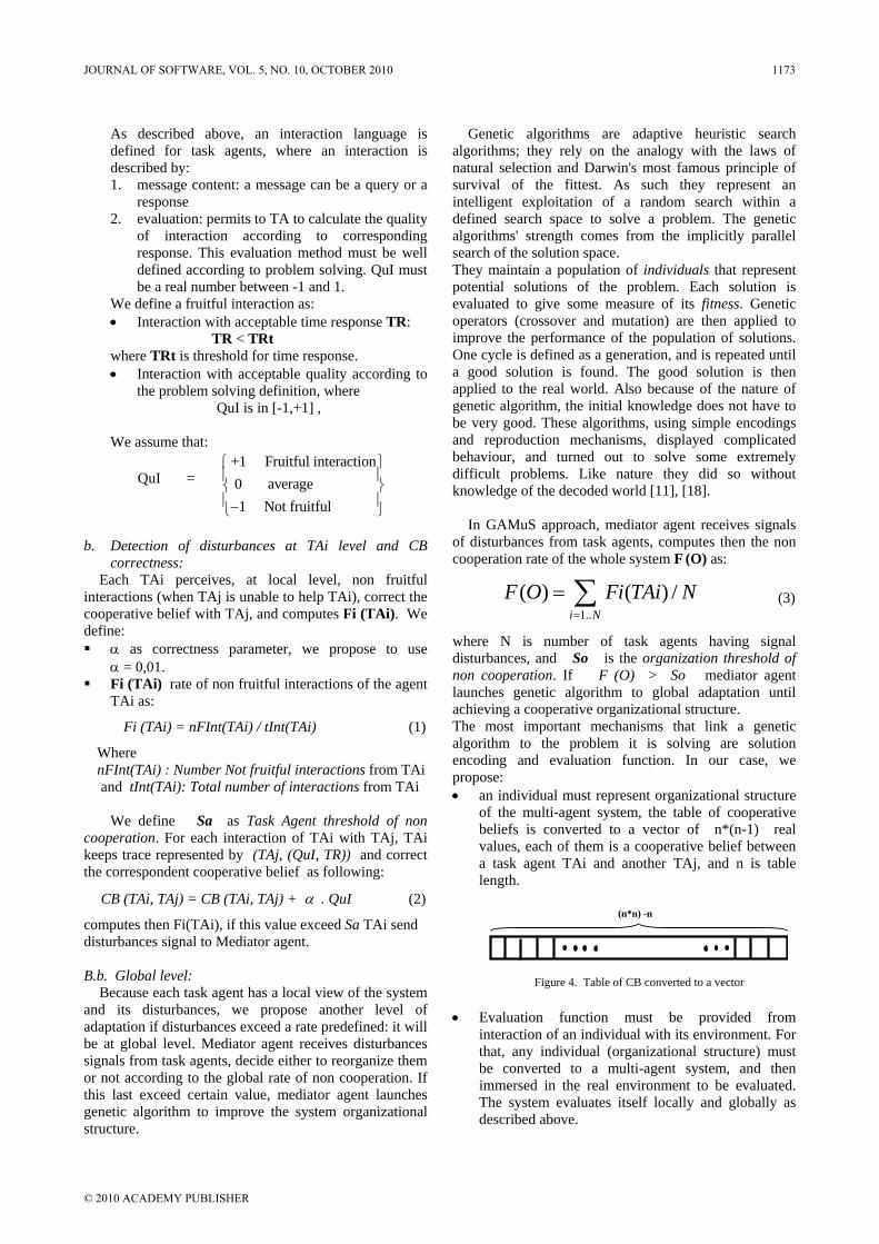
As described above, an interaction language is defined for task agents, where an interaction is described by: 1. message content: a message can be a query or a

response 2. evaluation: permits to TA to calculate the quality

of interaction according to corresponding response. This evaluation method must be well defined according to problem solving. QuI must be a real number between -1 and 1.

We define a fruitful interaction as: • Interaction with acceptable time response TR:

TR < TRt where TRt is threshold for time response. • Interaction with acceptable quality according to

the problem solving definition, where QuI is in [-1,+1] ,

We assume that:

QuI = +1 Fruitful interaction 0 average

1 Not fruitful

⎧ ⎫⎪ ⎪⎨ ⎬⎪ ⎪−⎩ ⎭

b. Detection of disturbances at TAi level and CB

correctness: Each TAi perceives, at local level, non fruitful

interactions (when TAj is unable to help TAi), correct the cooperative belief with TAj, and computes Fi (TAi). We define: α as correctness parameter, we propose to use

α = 0,01. Fi (TAi) rate of non fruitful interactions of the agent

TAi as:

Fi (TAi) = nFInt(TAi) / tInt(TAi) (1)

Where nFInt(TAi) : Number Not fruitful interactions from TAi and tInt(TAi): Total number of interactions from TAi

We define Sa as Task Agent threshold of non

cooperation. For each interaction of TAi with TAj, TAi keeps trace represented by (TAj, (QuI, TR)) and correct the correspondent cooperative belief as following:

CB (TAi, TAj) = CB (TAi, TAj) + α . QuI (2)

computes then Fi(TAi), if this value exceed Sa TAi send disturbances signal to Mediator agent. B.b. Global level:

Because each task agent has a local view of the system and its disturbances, we propose another level of adaptation if disturbances exceed a rate predefined: it will be at global level. Mediator agent receives disturbances signals from task agents, decide either to reorganize them or not according to the global rate of non cooperation. If this last exceed certain value, mediator agent launches genetic algorithm to improve the system organizational structure.

Genetic algorithms are adaptive heuristic search algorithms; they rely on the analogy with the laws of natural selection and Darwin's most famous principle of survival of the fittest. As such they represent an intelligent exploitation of a random search within a defined search space to solve a problem. The genetic algorithms' strength comes from the implicitly parallel search of the solution space. They maintain a population of individuals that represent potential solutions of the problem. Each solution is evaluated to give some measure of its fitness. Genetic operators (crossover and mutation) are then applied to improve the performance of the population of solutions. One cycle is defined as a generation, and is repeated until a good solution is found. The good solution is then applied to the real world. Also because of the nature of genetic algorithm, the initial knowledge does not have to be very good. These algorithms, using simple encodings and reproduction mechanisms, displayed complicated behaviour, and turned out to solve some extremely difficult problems. Like nature they did so without knowledge of the decoded world [11], [18].

In GAMuS approach, mediator agent receives signals of disturbances from task agents, computes then the non cooperation rate of the whole system F (O) as:

1..

( ) ( ) /i N

F O Fi TAi N=

= ∑ (3)

where N is number of task agents having signal disturbances, and So is the organization threshold of non cooperation. If F (O) > So mediator agent launches genetic algorithm to global adaptation until achieving a cooperative organizational structure. The most important mechanisms that link a genetic algorithm to the problem it is solving are solution encoding and evaluation function. In our case, we propose: • an individual must represent organizational structure

of the multi-agent system, the table of cooperative beliefs is converted to a vector of n*(n-1) real values, each of them is a cooperative belief between a task agent TAi and another TAj, and n is table length.

• Evaluation function must be provided from

interaction of an individual with its environment. For that, any individual (organizational structure) must be converted to a multi-agent system, and then immersed in the real environment to be evaluated. The system evaluates itself locally and globally as described above.

(n*n) -n

Figure 4. Table of CB converted to a vector



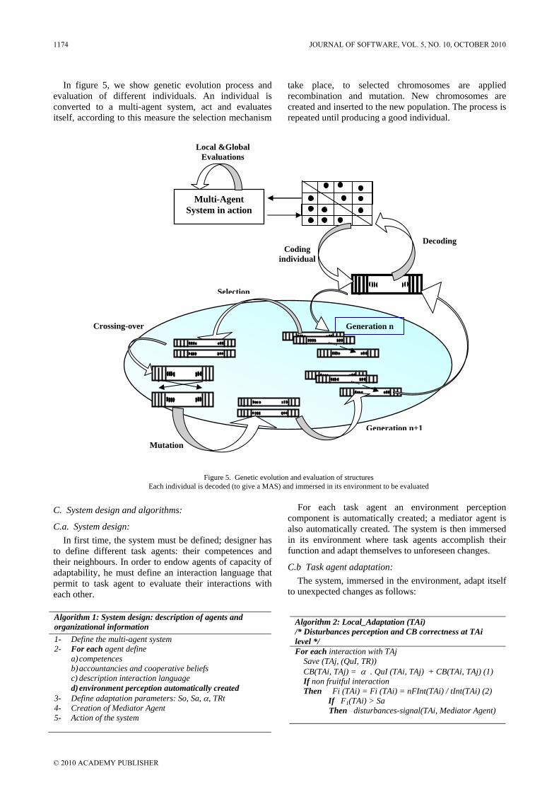
In figure 5, we show genetic evolution process and evaluation of different individuals. An individual is converted to a multi-agent system, act and evaluates itself, according to this measure the selection mechanism

take place, to selected chromosomes are applied recombination and mutation. New chromosomes are created and inserted to the new population. The process is repeated until producing a good individual.

C. System design and algorithms:

C.a. System design: In first time, the system must be defined; designer has

to define different task agents: their competences and their neighbours. In order to endow agents of capacity of adaptability, he must define an interaction language that permit to task agent to evaluate their interactions with each other.

For each task agent an environment perception component is automatically created; a mediator agent is also automatically created. The system is then immersed in its environment where task agents accomplish their function and adapt themselves to unforeseen changes.

C.b Task agent adaptation: The system, immersed in the environment, adapt itself

to unexpected changes as follows:

Figure 5. Genetic evolution and evaluation of structures Each individual is decoded (to give a MAS) and immersed in its environment to be evaluated

Decoding

Generation n

Selection

Crossing-over

Mutation Generation n+1

Multi-Agent System in action

Coding individual

Local &Global Evaluations

Algorithm 1: System design: description of agents and organizational information 1- Define the multi-agent system 2- For each agent define

a) competences b) accountancies and cooperative beliefs c) description interaction language d) environment perception automatically created

3- Define adaptation parameters: So, Sa, α, TRt 4- Creation of Mediator Agent 5- Action of the system

Algorithm 2: Local_Adaptation (TAi) /* Disturbances perception and CB correctness at TAi level */ For each interaction with TAj

Save (TAj, (QuI, TR)) CB(TAi, TAj) = α . QuI (TAi, TAj) + CB(TAi, TAj) (1) If non fruitful interaction Then Fi (TAi) = Fi (TAi) = nFInt(TAi) / tInt(TAi) (2)

If F1(TAi) > Sa Then disturbances-signal(TAi, Mediator Agent)



C.c. Action of mediator agent Reorganization of task agents is fulfilled by mediator agent as follows:

Evaluation of individuals: each individual is decoded to real multi-agent system, the set of cooperative beliefs represent links between agents, and then it is immersed in its environment and evaluated.

IV. EXPERIMENTATION AND RESULTS

We have implemented an adaptive system with JADE platform (Java Agent DEvelopment framework), JADE is a software development framework aimed at developing multi-agent systems and applications conforming to FIPA standards for intelligent agents. JADE is completely written in JAVA. The agent platform can be distributed across machines, it offers possibility to create multiple containers, and each container can be implemented on a machine [14]. Figure 6 shows Jade platform architecture.

A system developed with Jade platform must have at least the main container which contains necessary Directory Facilitator agent (DF) that provides a yellow pages service, Agent Management System agent (AMS) that ensures that each agent in the platform has a unique name.

We have implemented a simulation of an adaptive

system, composed of mediator agent and 15 task agents. The mediator agent has been created in the main container and the task agents in another one (container1). The figure below shows sniffer agent generated automatically by Jade platform. This agent shows at the right side interactions between system agents and their containers at the left one.

In a first time, we have experimented global adaptation process. Preliminary results that we have obtained are presented in figure 8. Graphs represent evolution of system evaluation according to algorithm 4. Mediator agent must minimize non cooperation rate of the system to a value predefined named So.

Figure 8.a shows system evaluation in the case of population size =500, mutation rate = 0.02 and selection rate = 60% and So = 0.18.

Figure 8.b shows system evaluation in the case of population size =500, mutation rate = 0.02 and selection rate = 60% and So =0.35.

Figure 6. JADE platform architecture

Figure 7. Jade sniffer agent. This shows a communication between

Mediator Agent(Main Container) and 3 Task Agents (Container 1)

Algorithm 4 : Evaluation(Oi) /*Evaluation of organization i*/

a) Convert a vector of CB to a MAS b) Action in the environment c) Observe the corresponding system behavior d) Evaluate organization cooperation

for each TAi /*Local level */ Fi (TAi) = nFInt(TAi) / tInt(TAi) (1)

Global level at Mediator Agent

1..

( ) ( ) /i N

F O Fi TAi N=

= ∑ (3)

Algorithm 3 Global_Adaptation (Fi(Ai)) /* Reorganization action of the Mediator Agent */ I-/

1..( ) ( ) /

i NF O Fi TAi N

=

= ∑ (3)

II-/ If F(O) > So then 1. Initialize algorithm parameters /* Population size, mutation rate, crossover rate*/ 2. Initialize the population; /* each individual is a vector of table of cooperative beliefs represented as vector of reals*/ 3. For each individual (organizational structure)

a) Evaluation b) Selection c) Reproduction (crossing-over and mutation)

4. GO to 3- until observe a cooperative organizational structure

Where F(O) < So



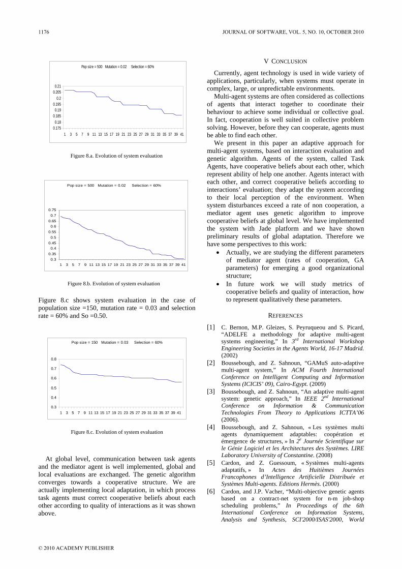
Figure 8.c shows system evaluation in the case of population size =150, mutation rate = 0.03 and selection rate = 60% and So =0.50.

At global level, communication between task agents and the mediator agent is well implemented, global and local evaluations are exchanged. The genetic algorithm converges towards a cooperative structure. We are actually implementing local adaptation, in which process task agents must correct cooperative beliefs about each other according to quality of interactions as it was shown above.

V CONCLUSION

Currently, agent technology is used in wide variety of applications, particularly, when systems must operate in complex, large, or unpredictable environments.

Multi-agent systems are often considered as collections of agents that interact together to coordinate their behaviour to achieve some individual or collective goal. In fact, cooperation is well suited in collective problem solving. However, before they can cooperate, agents must be able to find each other.

We present in this paper an adaptive approach for multi-agent systems, based on interaction evaluation and genetic algorithm. Agents of the system, called Task Agents, have cooperative beliefs about each other, which represent ability of help one another. Agents interact with each other, and correct cooperative beliefs according to interactions’ evaluation; they adapt the system according to their local perception of the environment. When system disturbances exceed a rate of non cooperation, a mediator agent uses genetic algorithm to improve cooperative beliefs at global level. We have implemented the system with Jade platform and we have shown preliminary results of global adaptation. Therefore we have some perspectives to this work:

• Actually, we are studying the different parameters of mediator agent (rates of cooperation, GA parameters) for emerging a good organizational structure;

• In future work we will study metrics of cooperative beliefs and quality of interaction, how to represent qualitatively these parameters.

REFERENCES

[1] C. Bernon, M.P. Gleizes, S. Peyruqueou and S. Picard, “ADELFE a methodology for adaptive multi-agent systems engineering,” In 3rd International Workshop Engineering Societies in the Agents World, 16-17 Madrid. (2002)

[2] Boussebough, and Z. Sahnoun, “GAMuS auto-adaptive multi-agent system,” In ACM Fourth International Conference on Intelligent Computing and Information Systems (ICICIS’ 09), Cairo-Egypt. (2009)

[3] Boussebough, and Z. Sahnoun, “An adaptive multi-agent system: genetic approach,” In IEEE 2nd International Conference on Information & Communication Technologies From Theory to Applications ICTTA’06 (2006).

[4] Boussebough, and Z. Sahnoun, « Les systèmes multi agents dynamiquement adaptables: coopération et émergence de structures, » In 2e Journée Scientifique sur le Génie Logiciel et les Architectures des Systèmes. LIRE Laboratory University of Constantine. (2008)

[5] Cardon, and Z. Guessoum, « Systèmes multi-agents adaptatifs, » In Actes des Huitièmes Journées Francophones d’Intelligence Artificielle Distribuée et Systèmes Multi-agents. Editions Hermès. (2000)

[6] Cardon, and J.P. Vacher, “Multi-objective genetic agents based on a contract-net system for n-m job-shop scheduling problems,” In Proceedings of the 6th International Conference on Information Systems, Analysis and Synthesis, SCI'2000/ISAS'2000, World

Pop size = 500 Mutation = 0.02 Selection = 60%

0.30.350.4

0.450.5

0.550.6

0.650.7

0.75

1 3 5 7 9 11 13 15 17 19 21 23 25 27 29 31 33 35 37 39 41

Figure 8.b. Evolution of system evaluation


0.1750.18

0.1850.19

0.1950.2

0.2050.21

1 3 5 7 9 11 13 15 17 19 21 23 25 27 29 31 33 35 37 39 41

Figure 8.a. Evolution of system evaluation


0.3

0.4

0.5

0.6

0.7

0.8

1 3 5 7 9 11 13 15 17 19 21 23 25 27 29 31 33 35 37 39 41

Figure 8.c. Evolution of system evaluation



Multiconference on Systemics, Cybernetics and Informations. (2000)

[7] Cardon, « Conscience artificielle & systèmes adaptatifs » Chapters 14, 15, 16, Ed. Eyrolles. (2000)

[8] S.A. DeLoach, “Organizational model for adaptive complex systems,” In Virginia Dignum (ed.) Multi-Agent Systems: Semantics and Dynamics of Organizational Models. IGI Global: Hershey, PA (2009). ISBN: 1-60566-256-9.

[9] J. Ferber, T. Stratulat and J. Tranier “Towards an integral approach of organizations in multi-agent systems: the MASQ approach,” In Multi-agent Systems: Semantics and Dynamics of Organizational Models in Virginia Dignum (Ed), IGI (2009).

[10] M.P. Gleizes, V. Camps and P. Glize “A theory of emergent computation based on cooperative self-organization for adaptive artificial systems,” In 4thEuropean Congress of Systems Science, Valencia. (1999)

[11] D. Goldberg “Algorithmes génétiques,” In Addison Wesley. (1994)

[12] Z. Guessoum, J.P. Briot, O. Marin, A. Hamel and P. Sens, “Dynamic and adaptive replication for large-scale reliable multi-agent systems,” In LNCS 2603, pp. 182–198. Springer-Verlag Berlin Heidelberg. (2003)

[13] T.D. Haynes and S. Sen, “Co-adaptation in a team,” In International Journal of Computational Intelligence and Organization, Vol 14, 1-20, New Jersey (1997), USA.

[14] Jade (2006), « Jade tutorial » available at http://jade.tilab.com.

[15] C.Oh. Jae “Emergence of cooperative internet server sharing among internet search agents caught in the n-Person prisoner’s dilemma game,” In Knowledge and Information Systems 2004.

[16] M.A. Florea, E. Kaliz and C. Carabelea “Genetic prediction of a multi-agent environment evolution,” CASYS’ 2000, Liege, Belgium, 7-12.

[17] V.F. Martinez and E. Sklar “A team-based co-evolutionary approach to multi-agent learning,” In Workshop Proceeding of 3rd International Conference on Autonomous Agents and MAS 2004.

[18] Z. Michalewicz “Genetic algorithms + data structures = evolution programs,” 3rd edition, Springer-Verlag, Berlin 1996.

[19] G. Picard, C. Bernon and M.P. Gleizes “Cooperative agent model within ADELFE framework: an application

to a timetabling problem,” In AAMAS'04, New York, USA 2004.

[20] Spector and A. Robinson “Multi-type, self-adaptive genetic programming as an agent creation tool,” In Workshop on Evolutionary Computation for Multi-Agent Systems, ECOMAS-2002, International Society for Genetic and Evolutionary Computation.

[21] K.P. Sycara “Multiagent systems,” In AI magazine Volume 19, No.2 Intelligent Agents Summer1998.

[22] J.M. Vidal “Fundamentals of multiagent systems with NetLogo examples” Copyright © 2006.

Imane Boussebough is a PHd student of computer science in the Department of computer science at university of Mentouri (Constantine, Algeria), received the ingéniorat and MS degrees both in Computer Science from university of Mentouri. She is member of the software engineering and artificial intelligence research team. Her research interests are in the areas of adaptive systems, multi agents systems, Web information research and filtering and complex systems. Ramdane Maamri is an associate Professor of computer science in the Department of computer science at university of Mentouri (Constantine, Algeria), received his Ingéniorat from university of Mentouri, MS in computer science from the University of Minnesota (USA), and PhD in computer science from university of Mentouri. He is the responsible of mathematics and computer science field at University of Mentouri and he leads the software engineering and artificial intelligence research team. His research interests are in the areas of intelligent agent and multi-agent systems, component based software development and reuse, fuzzy ontologies, Web services, artificial intelligence, and software testing. Zaidi Sahnoun is a professor of computer science at the Department of Computer Science of the University of Mentouri of Constantine in Algeria. He holds a Ph.D. in information technology from Rensselaer Polytechnic Institute in U.S.A. His main areas of interest include software engineering, formal methods, multi agent systems and complex systems.



Call for Papers and Special Issues

Aims and Scope. Journal of Software (JSW, ISSN 1796-217X) is a scholarly peer-reviewed international scientific journal focusing on theories, methods, and

applications in software. It provide a high profile, leading edge forum for academic researchers, industrial professionals, engineers, consultants, managers, educators and policy makers working in the field to contribute and disseminate innovative new work on software.

We are interested in well-defined theoretical results and empirical studies that have potential impact on the construction, analysis, or management

of software. The scope of this Journal ranges from the mechanisms through the development of principles to the application of those principles to specific environments. JSW invites original, previously unpublished, research, survey and tutorial papers, plus case studies and short research notes, on both applied and theoretical aspects of software. Topics of interest include, but are not restricted to:

• Software Requirements Engineering, Architectures and Design, Development and Maintenance, Project Management, • Software Testing, Diagnosis, and Validation, Software Analysis, Assessment, and Evaluation, Theory and Formal Methods • Design and Analysis of Algorithms, Human-Computer Interaction, Software Processes and Workflows • Reverse Engineering and Software Maintenance, Aspect-Orientation and Feature Interaction, Object-Oriented Technology • Component-Based Software Engineering, Computer-Supported Cooperative Work, Agent-Based Software Systems, Middleware Techniques • AI and Knowledge Based Software Engineering, Empirical Software Engineering and Metrics • Software Security, Safety and Reliability, Distribution and Parallelism, Databases • Software Economics, Policy and Ethics, Tools and Development Environments, Programming Languages and Software Engineering • Mobile and Ubiquitous Computing, Embedded and Real-time Software, Database, Data Mining, and Data Warehousing • Internet and Information Systems Development, Web-Based Tools, Systems, and Environments, State-Of-The-Art Survey

Special Issue Guidelines Special issues feature specifically aimed and targeted topics of interest contributed by authors responding to a particular Call for Papers or by

invitation, edited by guest editor(s). We encourage you to submit proposals for creating special issues in areas that are of interest to the Journal. Preference will be given to proposals that cover some unique aspect of the technology and ones that include subjects that are timely and useful to the readers of the Journal. A Special Issue is typically made of 10 to 15 papers, with each paper 8 to 12 pages of length.

The following information should be included as part of the proposal: • Proposed title for the Special Issue • Description of the topic area to be focused upon and justification • Review process for the selection and rejection of papers. • Name, contact, position, affiliation, and biography of the Guest Editor(s) • List of potential reviewers • Potential authors to the issue • Tentative time-table for the call for papers and reviews If a proposal is accepted, the guest editor will be responsible for: • Preparing the “Call for Papers” to be included on the Journal’s Web site. • Distribution of the Call for Papers broadly to various mailing lists and sites. • Getting submissions, arranging review process, making decisions, and carrying out all correspondence with the authors. Authors should be

informed the Instructions for Authors. • Providing us the completed and approved final versions of the papers formatted in the Journal’s style, together with all authors’ contact

information. • Writing a one- or two-page introductory editorial to be published in the Special Issue.

Special Issue for a Conference/Workshop A special issue for a Conference/Workshop is usually released in association with the committee members of the Conference/Workshop like

general chairs and/or program chairs who are appointed as the Guest Editors of the Special Issue. Special Issue for a Conference/Workshop is typically made of 10 to 15 papers, with each paper 8 to 12 pages of length.

Guest Editors are involved in the following steps in guest-editing a Special Issue based on a Conference/Workshop: • Selecting a Title for the Special Issue, e.g. “Special Issue: Selected Best Papers of XYZ Conference”. • Sending us a formal “Letter of Intent” for the Special Issue. • Creating a “Call for Papers” for the Special Issue, posting it on the conference web site, and publicizing it to the conference attendees.

Information about the Journal and Academy Publisher can be included in the Call for Papers. • Establishing criteria for paper selection/rejections. The papers can be nominated based on multiple criteria, e.g. rank in review process plus

the evaluation from the Session Chairs and the feedback from the Conference attendees. • Selecting and inviting submissions, arranging review process, making decisions, and carrying out all correspondence with the authors.

Authors should be informed the Author Instructions. Usually, the Proceedings manuscripts should be expanded and enhanced. • Providing us the completed and approved final versions of the papers formatted in the Journal’s style, together with all authors’ contact

information. • Writing a one- or two-page introductory editorial to be published in the Special Issue. More information is available on the web site at http://www.academypublisher.com/jsw/.

(Contents Continued from Back Cover)

REGULAR PAPERS Multiprocessor Scheduling by Simulated Evolution Imtiaz Ahmad, Muhammad K. Dhodhi, and Ishfaq Ahmad The Chinese Text Categorization System with Category Priorities Huan-Chao Keh, Ding-An Chiang, Chih-Cheng Hsu, and Hui-Hua Huang A Pre-Injection Analysis for Identifying Fault-Injection Tests for Protocol Validation Neeraj Suri and Purnendu Sinha The Use of AHP in Security Policy Decision Making: An Open Office Calc Application Irfan Syamsuddin and Junseok Hwang Adaptive Multi-agent System: Cooperation and Structures Emergence Imane Boussebough, Ramdane Maamri, Zaïdi Sahnoun

1128

1137

1144

1162

1170

A-study-on-framework-and-realizing-mechanism-of-ISEE ...

Documents

Transcript of A-study-on-framework-and-realizing-mechanism-of-ISEE ...