A New And Improved Version Of HULLAC

A New And Improved Version Of HULLAC

M. Klapischa , M. Busqueta,b and A. Bar-Shaloma,c

aARTEP#,inc. 2922 Excelsior Springs Court, Ellicott City, MD 21042,USA bLERMA, Observatoire de Paris, UPMC, CNRS, Place Jules Janssen, 92190 Meudon, France

cNRCN, 9001 Be’er Sheva, Israel.

Abstract: We present a new version of the collisional radiative model (CRM) generator code HULLAC. The main features are: (i) input considerably simplified and flexible, (ii) capacity of “post-averaging” configurations and superconfigurations in mixed mode, (iii) a new fitting formula for cross sections, completely correcting the problems of the classical Sampson and Golden formula, (iv) a new algorithm for solving the rate equations of the CRM, more robust and giving more insight in the quality of the model than the biconjugate gradient method, (v) thanks to thorough comparisons with the LANL code, some errors were corrected, and very good agreement has been obtained on all types of transitions, (vi) finally, most of the code has been re-written according to up-to-date standards. This code is now ready for distribution. Keywords: Non-LTE, collisional radiative model, collisional cross sections, rate equation solver. PACS: 33.20Rm, 52.20Fs, 52.25Dg, 52.25Os.

INTRODUCTION

The HULLAC code [1] is an integrated collisional radiative model generator and solver. Its efficiency is due to original methods and algorithms. All relevant processes are computed with the same relativistic wavefunctions [2]. The angular momentum recoupling coefficients are computed using graphical methods [3]. The collision processes use the factorization-linearization method [4],[5]. It has been used by a number of groups, and was advertised at the 2001 APIP [6]. However, because the different modules were developed over the years, most of the coding was obsolescent. This is why it was decided to rewrite1 most of the code in a modern style, more conform to standards of software engineering, in order for the code source to be understood and compiled easily by potential users. By the same token, many improvements have been made, and errors have been corrected. The rate equation solver, which was missing in previous versions, has been developed, based on a new algorithm. It is the purpose of this paper to describe these improvements and additions. The reader is referred to the above references for the theory.

to whom correspondence should be addressed: [email protected] # Contractor to Naval Research Laboratory, Washington, DC, 20375. 1 mostly done by M.B.

206

Downloaded 25 Sep 2007 to 132.250.22.4. Redistribution subject to AIP license or copyright, see http://proceedings.aip.org/proceedings/cpcr.jsp

NEW INPUT POSSIBILITIES

The module anglar acts as the master module, in addition to computing all the angular momentum coefficients of the various matrix elements of the energy and of all the transitions, spontaneous and collisional. It reads an input file in which, among other data, the list of configurations to be computed should be listed. This was inefficient and painstaking for complex spectra.

Defining Configurations

It is now possible to use the concept of superconfigurations [7] to generate all the desired configurations in a very compact manner.

FIGURE 1. Flow chart of the HULLAC package. AME stands for angular matrix elements.

For instance, the following lines:

superconf nel=15 abc 1s2 2L [5:8] 3L [0:18] (4L,5L) [0:1]

endsuper generate all and only those configurations with a total of 15 electrons distributed between the supershells (2s,2p) – with all combinations from 5 to 8 electrons, (3s,3p,3d) – with zero to 18 electrons, and (4s,4p,4d,4f,5s,5p,5d,5f,5g) supershell with 0 to 1 electron. As a new addition, the symbols “Le” and “Lo” would select only even or odd values of l . The sizes of the arrays have been greatly increased to do very complex computations, but if there is an overflow, it will now be detected and the relevant parameter will be clearly designated in the output file.

207


Choosing Potentials

There was in nearly all versions of HULLAC the possibility of computing different groups of configurations in different potentials. This can greatly increase the accuracy of the energies and wavefunctions. This is now achieved in a very simple way with the keyword: potential new. In the same way, the potential to be chosen as the final one – with respect to which the other configurations are shifted to take into account their accurate computations – is simply designated as potential new final.

“Direct-“ and “Post-“ Averaging

In the previous versions, all the input configurations created a list of fine structure levels in jj coupling. For complex spectra, this generates too many detailed levels. Therefore, several modes were introduced in the SETTING chapter of the input file:

mode = l(evels) – this generates as before fine structure levels for all configurations listed.

mode = c(onfigurations) – this generates directly, by simple sum rules, relativistic configuration averages as basic entities for the whole chain of program. mode = l+c – makes two sets of output files for all the rates, and two different solutions can be obtained at the level of the CRM solver “colrad”.

In addition, one can now perform “post averaging”, that is, anglar generates one of the two previous sets, but can then perform additional, “brute force” averaging. Since anglar is the less time consuming module of the chain, it is not a significant penalty. Two additional keywords are possible: nrc - creates non relativistic configurations averages (NRC) of relativistic configurations by statistical weight, and sc - creates superconfigurations as averages of configurations. These two averages can be done starting from mode c or l. In the latter case, the effects of configuration interaction will be included in the averages. These averages can be performed on all the levels or configurations in the list, or on selected levels/configurations, in effect creating a “mixed model” in which some configurations can be described as fine structure levels, others a configuration averages, and some others as superconfigurations. The reader is referred to the mode of use for more details

A NEW FITTING FORMULA

Collisional excitation cross sections are the most time-consuming part of setting the model. The temperature dependent rates are obtained by integrating them over the collision energy. Therefore, it is has become standard to represent the cross sections by an easily integrable analytical formula, the parameters of which are transmitted from the cross section module to the CRM equation solver module, so the same cross sections can be used to model several temperatures. The classical, nearly ubiquitous, formula is usually called the “Golden and Sampson (GS) formula”[8].

It reads:

!(u = " / #E) = A + D ln(u) + c1

(a + u)+

c2

(a + u)2

,

208


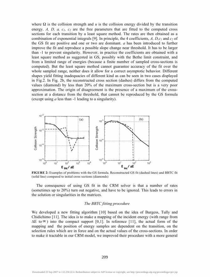
where Ω is the collision strength and u is the collision energy divided by the transition energy. A, D, a, c1, c2 are the free parameters that are fitted to the computed cross sections for each transition by a least square method. The rates are then obtained as a combination of exponential integrals [9]. In principle, the 4 coefficients, A, D,c1 and c2 of the GS fit are positive and one or two are dominant. a has been introduced to further improve the fit and reproduce a possible slope change near threshold. It has to be larger than -1 to prevent singularity. However, in practice the coefficients are obtained with a least square method as suggested in GS, possibly with the Bethe limit constraint, and from a limited range of energies (because a finite number of sampled cross-sections is computed). But the least square method cannot guarantee accuracy of the fit over the whole sampled range, neither does it allow for a correct asymptotic behavior. Different shapes yield fitting inadequacies of different kind as can be seen in two cases displayed in Fig.2. In Fig. 2b, the reconstructed cross section (dashes) differs from the computed values (diamond) by less than 20% of the maximum cross-section but is a very poor approximation. The origin of disagreement is the presence of a maximum of the cross-section at a distance from the threshold, that cannot be reproduced by the GS formula (except using a less than -1 leading to a singularity).

10-5

10-4

10-3

10-2

100

101

102

103

104

Colli

sion S

trength

E inc / !E

(a)

10-5

10-4

10-3

100

101

102

103

E inc

/ !E

Colli

sion S

trength

(b)

FIGURE 2: Examples of problems with the GS formula. Reconstructed GS fit (dashed lines) and BBTC fit (solid line) compared to initial cross sections (diamonds)

The consequence of using GS fit in the CRM solver is that a number of rates

(sometimes up to 20%) turn out negative, and have to be ignored. This leads to errors in the solution or singularities in the matrices.

The BBTC fitting procedure

We developed a new fitting algorithm [10] based on the idea of Burgess, Tully and Chidichimo [11]. The idea is to make a mapping of the incident energy (with range from ∆E to! ) into the compact support [0,1]. In reference [11], the actual form of the mapping and the position of energy samples are dependent on the transition, on the selection rules which are in force and on the actual values of the cross-sections. In order to make it tractable in our CRM model, we improved their procedure with a more general

209


procedure and a fixed, optimized set of sampling point. We map the function !(u) to a function z(x) with the following transformation:

x = 1! (1+ C) / (u + C),

z = ("! A lnu).(u + C)n.

here n is the integer power of the residue (i.e. after the logarithmic term has been taken out) obtained from the asymptotic behavior deduced from the last 2 or 3 computed cross-sections, and C is a free parameter to optimize the fit. The collision strength then reads:

! = A lnu + z / (u + C)n.

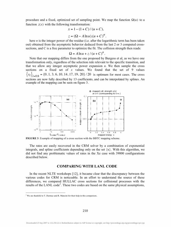
Note that our mapping differs from the one proposed by Burgess et al, as we have one transformation only, regardless of the selection rule relevant to the specific transition, and that we allow any integer asymptotic power expansion n. We then sample the cross sections on a fixed set of x values. We found that the set of 9 values xl{ }

l=0:8= {0,!1,!3,!6,!10,!14,!17,!19,!20} / 20 is optimum for most cases. The cross

sections are now fully described by 13 coefficients, and can be interpolated by splines. An example of the mapping can be seen on figure 3.

FIGURE 3: Example of mapping of a cross section with the BBTC mapping scheme.

The rates are easily recovered in the CRM solver by a combination of exponential

integrals, and spline coefficients depending only on the set {x}. With this algorithm, we did not find any problematic values of rates in the Xe case with 39000 configurations described below.

COMPARING WITH LANL CODE

In the recent NLTE workshops [12], it became clear that the discrepancy between the various codes for CRM is noticeable. In an effort to understand the source of these differences, we compared HULLAC cross sections for collisional processes with the results of the LANL code2. These two codes are based on the same physical assumptions,

2 We are thankful to T. Durmaz and R. Mancini for their help in this comparison.

210


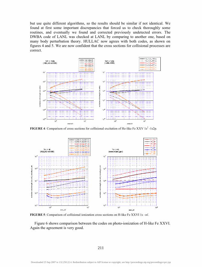
but use quite different algorithms, so the results should be similar if not identical. We found at first some important discrepancies that forced us to check thoroughly some routines, and eventually we found and corrected previously undetected errors. The DWBA code of LANL was checked at LANL by comparing to another one, based on many body perturbation theory. HULLAC now agrees with both codes, as shown on figures 4 and 5. We are now confident that the cross sections for collisional processes are correct.

FIGURE 4: Comparison of cross sections for collisional excitation of He-like Fe XXV 1s2 -1s2p.

FIGURE 5: Comparison of collisional ionization cross sections on H-like Fe XXVI 1s –nl.

Figure 6 shows comparison between the codes on photo-ionization of H-like Fe XXVI.

Again the agreement is very good.

211


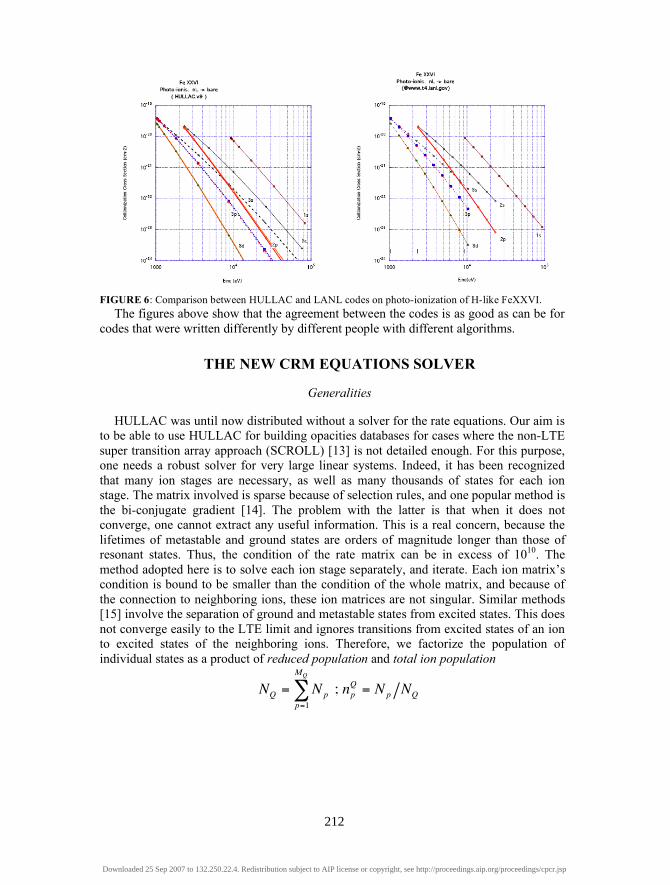
FIGURE 6: Comparison between HULLAC and LANL codes on photo-ionization of H-like FeXXVI.

The figures above show that the agreement between the codes is as good as can be for codes that were written differently by different people with different algorithms.

THE NEW CRM EQUATIONS SOLVER

Generalities

HULLAC was until now distributed without a solver for the rate equations. Our aim is to be able to use HULLAC for building opacities databases for cases where the non-LTE super transition array approach (SCROLL) [13] is not detailed enough. For this purpose, one needs a robust solver for very large linear systems. Indeed, it has been recognized that many ion stages are necessary, as well as many thousands of states for each ion stage. The matrix involved is sparse because of selection rules, and one popular method is the bi-conjugate gradient [14]. The problem with the latter is that when it does not converge, one cannot extract any useful information. This is a real concern, because the lifetimes of metastable and ground states are orders of magnitude longer than those of resonant states. Thus, the condition of the rate matrix can be in excess of 1010. The method adopted here is to solve each ion stage separately, and iterate. Each ion matrix’s condition is bound to be smaller than the condition of the whole matrix, and because of the connection to neighboring ions, these ion matrices are not singular. Similar methods [15] involve the separation of ground and metastable states from excited states. This does not converge easily to the LTE limit and ignores transitions from excited states of an ion to excited states of the neighboring ions. Therefore, we factorize the population of individual states as a product of reduced population and total ion population

NQ = Np

p=1

MQ

! ; npQ= Np NQ

212


where Np, NQ, np are, respectively, individual population of state p, total population of charge Q, and reduced population of level p of charge state Q. The advantage of this factorization is that the global effective rates WQ!Q ' – i.e. temperature and density dependent contribution from an ion to another, depend only on the reduced population:

WQ!Q ' =1

NQ

NpWp! p '

p"Q

#$

%&

'

()

p '"Q '

# = npQWp! p '

p"Q

#p '"Q '

#

Therefore, if the reduced populations are found at a given iteration, the global rates can be computed. Then a matrix, the order of which is only the number of active charge states, i.e. about a dozen, can be easily set up and solved, giving the charge state distribution, i.e. the NQ of the next iteration. Using a Newton-style development, we find the increments of the reduced populations:

!nQ = "

1

NQ

!NQ 'M

Q

-1R

Q%nQ ' + !N

Q"M

Q

-1SQ%nQ" + !N

Q%nQ +M

Q

"1 %GQ{ }

where Q’=Q+1, Q’’=Q-1, RQ and SQ are, respectively, the rectangular matrices of recombination and ionization into ion Q, and MQ is the matrix of transitions inside ion Q, including losses to other ions on the diagonal.

%GQ is the vector of the residues for the

states at the previous iteration. More details can be found in reference [16].

Results

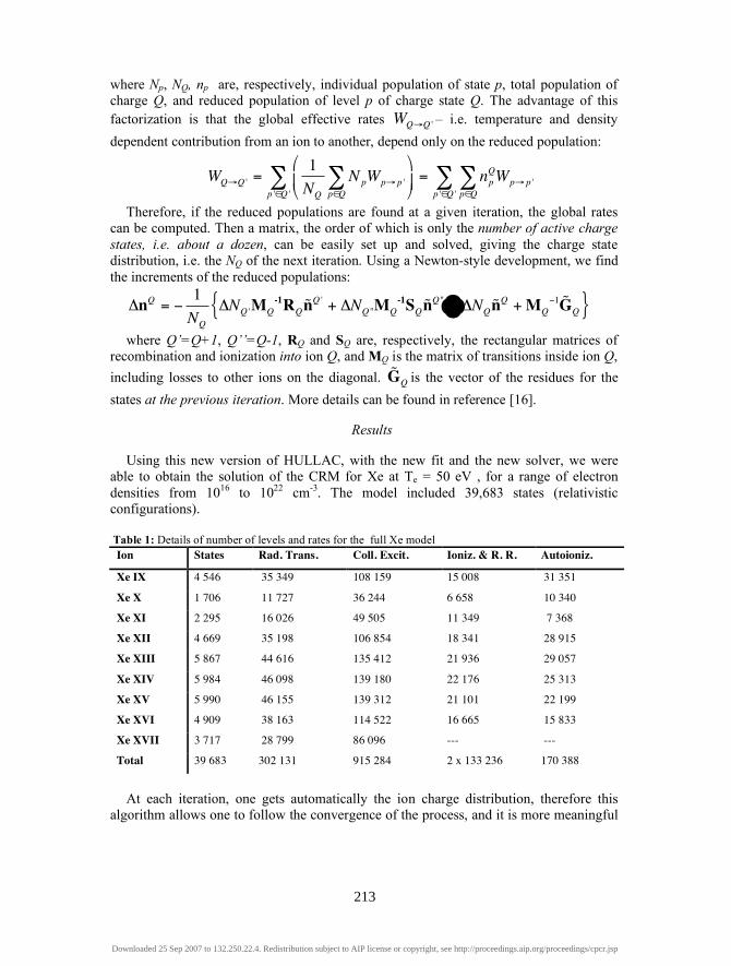
Using this new version of HULLAC, with the new fit and the new solver, we were able to obtain the solution of the CRM for Xe at Te = 50 eV , for a range of electron densities from 1016 to 1022 cm-3. The model included 39,683 states (relativistic configurations).

Table 1: Details of number of levels and rates for the full Xe model

Ion States Rad. Trans. Coll. Excit. Ioniz. & R. R. Autoioniz.

Xe IX 4 546 35 349 108 159 15 008 31 351

Xe X 1 706 11 727 36 244 6 658 10 340

Xe XI 2 295 16 026 49 505 11 349 7 368

Xe XII 4 669 35 198 106 854 18 341 28 915

Xe XIII 5 867 44 616 135 412 21 936 29 057

Xe XIV 5 984 46 098 139 180 22 176 25 313

Xe XV 5 990 46 155 139 312 21 101 22 199

Xe XVI 4 909 38 163 114 522 16 665 15 833

Xe XVII 3 717 28 799 86 096 --- ---

Total 39 683 302 131 915 284 2 x 133 236 170 388

At each iteration, one gets automatically the ion charge distribution, therefore this

algorithm allows one to follow the convergence of the process, and it is more meaningful

213


than a “black box” algorithm in which the iteration do not have physical meaning. It is then possible to stop at the required accuracy, and create a compact database of charge distribution. Figure 7 shows the evolution of the charge distribution of a smaller model (with 2386 non-relativistic configuration averages). In this case, the convergence criterion was very stringent, (10-4 relative variation of individual populations), to show the stability of the algorithm.

Figure 8 displays the spectra obtained from the full model (39,683 states) at two different densities. There is no statistical approximation besides the configuration

average.

FIGURE 7: Evolution of charge distribution for Xe at Te =50 eV and Ne=1020 cm-3

10-6

10-4

10-2

100

102

104

106

108

1010

Inte

nsi

ty

40035030025020015010050

h! (eV)

Ne = 1016

cm-3

Ne = 1022

cm-3

FIGURE 8: Spectra of Xe (39,683 states) at Te =50 eV and Ne=1016 and 1022 cm-3.

SUMMARY AND CONCLUSION

This new version of HULLAC is much more reliable, complete, and easy to use than the previous ones. It was thoroughly checked by comparison to the LANL codes with excellent agreement. The new fitting procedure guarantees a trustworthy evaluation of the rates in the CRM solver. The latter has been shown to be robust and to give insight into

10-9

10-8

10-7

10-6

10-5

10-4

10-3

10-2

10-1

fractio

n(Z)

10008006004002000

iteration #

ion8 ion9 ion10 ion11 ion12 ion13 ion14 ion15 ion16 ion17 10

-10

10-9

10-8

10-7

10-6

10-5

10-4

10-3

10-2

10-1

fracti

on(i

on)

161412108

ion

NQest NQ 100 NQ 200 NQ 500 NQ 1.e_4

214


the atomic model. All the code is in Fortran – mostly 77 and 95 compatible–, and it was successfully compiled on many platforms. It is now ready for distribution.

ACKNOWLEDGEMENTS

We thank Dr. S. Obenschain, Head of the Laser Plasma Branch (LPB) of the Naval Research Laboratory for his encouragements and support. This work was done under a contract with LPB through a grant from the USDOE. We are grateful to Prof. R Mancini and T. Durmaz for help with the LANL codes.

REFERENCES

1. A. Bar-Shalom, M Klapisch, and J Oreg, J. Quant. Spectros. Rad. Transf. 71, 169 - 88 (2001). 2. M Klapisch, Comput. Phys. Comm. 2, 239 -60 (1971); E. Koenig, Physica(Utrecht) 62, 393 (1972). 3. A. Bar-Shalom and M. Klapisch, Comput. Phys. Comm. 50, 375 - 93 (1988). 4. A. Bar-Shalom, M Klapisch, and J. Oreg, Phys. Rev. A. 38, 1773- 84 (1988). 5. J. Oreg, W. H. Goldstein, M Klapisch et al., Phys. Rev. A 44, 1750 (1991). 6. A. Bar-Shalom, M Klapisch, and J Oreg, presented at the 13th Int'l Conference on Atomic Processes in Plasmas,

Gatlinburg, TN, (2002), D R Schultz, F W Meyer, and F Ownby Eds., AIP Conference Proceedings, 635, 92 - 100.

7. A. Bar-Shalom, J. Oreg, W. H. Goldstein et al., Phys. Rev. A. 40, 3183 - 93 (1989). 8. L B Golden and D H Sampson, Astroph. J. Supp. 38, 19 (1978); L B Golden, R E H Clark, S J Goett et al., Astroph.

J. Supp. 45, 603 - 12 (1981); S J Goett, R E H Clark, and D H Sampson, Atomic Data Nuclear Data Tables 25, 185 (1980).

9. M Abramowitz and I A Stegun, Handbook of Mathematical Functions. (Dover Publications, New York, 1965). 10. M Busquet, High Ener. Dens. Phys. doi:10.1016/j.hedp.2007.01.007 (2007). 11. A Burgess and J A Tully, Astronom. & Astrophys. 254, 436 - 53 (1992); A Burgess, M. C. Chidichimo, and J A

Tully, Astronom. & Astrophys. Supp. 131, 145 - 52 (1998). 12. Y Ralchenko, R W Lee, and C Bowen, presented at the 14th APS Topical conference on Atomic Processes in

Plasmas, Santa Fe, NM, (2004), J. S. Cohen, S. Mazevet, and D. P. Kilcrease Eds., AIP conference proceedings, 730, 151 -160.

13. A Bar-Shalom, J Oreg, and M Klapisch, J. Quant. Spectros. Rad. Transf. 65, 43 (2000). 14. William H Press, Brian P Flannery, Saul A Teukolsky et al., Numerical Recipes in Fortran 77 :The art of scientific

computing., 2nd ed. (Cambridge University Press, Cambridge, UK, 1996). 15. S. D. Loch, C. J. Fontes, J. Colgan et al., Phys. Rev. E 69, 066405 (2004); M Busquet, J P Raucourt, and J C

Gauthier, J. Quant. Spectros. Rad. Transf. 54, 81 - 87 (1995). 16. M. Klapisch and M. Busquet, High Ener. Dens. Phys. 3, 143-148 (2007).

215


A New And Improved Version Of HULLAC

Documents

Transcript of A New And Improved Version Of HULLAC