
A method for ranking components importance in presence of epistemic uncertainties
22
1 A method for ranking components importance in presence of epistemic uncertainties P. Baraldi, E. Zio, M. Compare Energy Department, Polytechnic of Milan, Via Ponzio 34/3 20133 Milan, Italy [email protected] ABSTRACT: Importance Measures (IMs) are used to rank the contributions of components or basic events to the system performance, e.g. its reliability or risk. Most times, IMs are calculated without due account of the uncertainties in the model of the behavior of the system. The objective of this work is to investigate how uncertainties can influence IMs and to develop a method for giving them due account in the corresponding ranking of the components or basic events. The uncertainties considered in this work affect the model parameters values and are assumed to be described by probability density functions. The method for ranking the contributors to the system performance measure, is applied to the auxiliary feedwater system of a nuclear pressurized water reactor. 1 Introduction A most relevant outcome of a Probabilistic Safety Assessment (PSA) is the identification of the risk/safety importance of basic events or components. This allows tracing system bottlenecks and provides guidelines for effective actions of system improvements. To this aim, Importance Measures (IMs) are appropriately used to rank the contributions of components or basic events to the system performance, e.g. the system reliability or risk. IMs were initially introduced to assess the contribution of the components to the overall system reliability [1]; later different IMs have been introduced to address various aspects of reliability, safety and risk significance (Fussel-Vesely (FV), Criticality, Risk Achievement Worth (RAW) and Risk Reduction Worth (RRW)) [2]. On the other hand, uncertainties inevitably enter the modeling of the behavior of a system and it is customary in practice to categorize them into two types: aleatory and epistemic [3]. The former type (also referred to as irreducible, stochastic or random uncertainty) describes the inherent variation associated with the physical system or the environment (e.g. variation in atmospheric conditions, in fatigue life of compressor and turbine blades, etc.); the latter (also referred to as subjective or reducible uncertainty) is, instead, due to a lack of knowledge of quantities or processes of the system or the environment (e.g. lack of experimental data to characterize new materials and processes, poor understanding of coupled physics phenomena, poor
-
Upload
independent -
Category
Documents
-
view
1 -
download
0
Transcript of A method for ranking components importance in presence of epistemic uncertainties
1
A method for ranking components importance in presence of epistemic
uncertainties
P. Baraldi, E. Zio, M. Compare
Energy Department, Polytechnic of Milan, Via Ponzio 34/3 20133 Milan, Italy
ABSTRACT: Importance Measures (IMs) are used to rank the contributions of components or basic events to
the system performance, e.g. its reliability or risk. Most times, IMs are calculated without due account of the
uncertainties in the model of the behavior of the system. The objective of this work is to investigate how
uncertainties can influence IMs and to develop a method for giving them due account in the corresponding
ranking of the components or basic events. The uncertainties considered in this work affect the model parameters
values and are assumed to be described by probability density functions. The method for ranking the contributors
to the system performance measure, is applied to the auxiliary feedwater system of a nuclear pressurized water
reactor.
1 Introduction
A most relevant outcome of a Probabilistic Safety Assessment (PSA) is the identification of the risk/safety
importance of basic events or components. This allows tracing system bottlenecks and provides guidelines for
effective actions of system improvements. To this aim, Importance Measures (IMs) are appropriately used to
rank the contributions of components or basic events to the system performance, e.g. the system reliability or
risk.
IMs were initially introduced to assess the contribution of the components to the overall system reliability [1];
later different IMs have been introduced to address various aspects of reliability, safety and risk significance
(Fussel-Vesely (FV), Criticality, Risk Achievement Worth (RAW) and Risk Reduction Worth (RRW)) [2].
On the other hand, uncertainties inevitably enter the modeling of the behavior of a system and it is customary in
practice to categorize them into two types: aleatory and epistemic [3]. The former type (also referred to as
irreducible, stochastic or random uncertainty) describes the inherent variation associated with the physical
system or the environment (e.g. variation in atmospheric conditions, in fatigue life of compressor and turbine
blades, etc.); the latter (also referred to as subjective or reducible uncertainty) is, instead, due to a lack of
knowledge of quantities or processes of the system or the environment (e.g. lack of experimental data to
characterize new materials and processes, poor understanding of coupled physics phenomena, poor
2
understanding of accident initiating events, etc.). In practice, IMs are typically calculated without due account of
the uncertainties.
This work is aimed at investigating how uncertainties can influence IMs and how they can be accounted for in
the ranking of the basic events or components. The uncertainties here considered are of epistemic type on the
values of the parameters of the system model and are represented by probability density functions.
The paper is organized as follows. In Section 2, a method for comparing the uncertain importance measures of
two components is presented. In Section 3, two case studies of increasing complexity are described, the second
of which concerns the auxiliary feed water system of a nuclear pressurized water reactor and entails the
introduction of a procedure for efficiently performing the ranking. A comparison is offered between the
proposed procedure and a method previously presented in the literature [4]. Concluding remarks on the issue and
an outlook to further research needed for addressing it are provided in Section 4.
2 Comparing the importance of components in presence of uncertainties
The aim of this Section is to present a method for comparing the importance of two components A and B of an
hypothetical system in presence of uncertainty on the components performance parameters (e.g. reliabilities,
failure rates, repair rates etc.), which propagate through the system model leading to uncertainties in the system
performance (e.g., its reliability). In this scenario, importance measures calculations should reflect these
uncertainties and so should the ranking.
With respect to the uncertainty representation, in general when sufficiently informative data are available
probabilistic distributions are righteously used. For simplicity of illustration, uniformly distributed uncertainty is
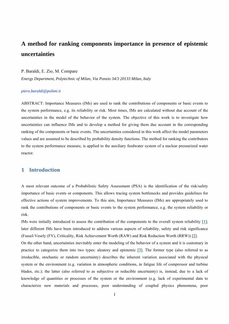
assumed to be affecting directly the IMs of components A and B. Table 1 reports the ranges of the IMs
distributions while Figure 1a and Figure 1b show the corresponding distributions. Looking at the distributions of
A and B IMs (denoted as and , respectively) one may observe that the IM of component B ( ) is
significantly more uncertain than that of component A ( ), but the expected value of , is greater than
that of B, . On the other hand, there is a range in which the quantiles are larger than the ones. For
example, if one were to perform the ranking based on the IMs 95th quantile values the conclusion would be that
component B is more important than A, contrarily to what would be happen if the ranking were based on the
expected values.
Table 1: Uniform distributions parameters.
Uniform distribution
Lower limit l Upper limit u
A 0.0141 0.0155
3
B 0.0020 0.0178
Figure 1: Probability density functions (pdfs) and cumulative distribution functions (cdfs) of the random variables , (a and
b) and (c and d) in case of IMs with uniformly distributed uncertainties.
The drawback of comparing the expected values or specific quantiles lies in the loss of information about the
distribution. With reference for example to Figure 1, the fact that the 95th quantile of (0.015) is lower than that
of (0.017) only means that the point value which is lower than with probability of 0.95 is lower than the
analogous point value for ; the full information on the actual difference between the distributions of and
does not play any role.
A natural way to give full account of the difference between the distributions of and is to consider the
random variable (rv) ‐ whose pdf and cdf are shown in Figure 1c and Figure 1d, respectively. The details on
their analytical expressions are given in Appendix 1. In order to establish if component A is more important than
B, one can consider the probability 1 0 that is greater than ; for example, in the present case
1 0 0.81, which means that with high probability component A is more important
than B.
To decide on the relative importance of the two components A and B, it is necessary to fix a threshold
0.5,1 on the value such that if is larger than T, then A is more important than B, otherwise no
conclusion can be given. Obviously, the lower the threshold, the higher the risk associated with the decision.
On the other hand, the choice of a simple-valued threshold has some limitations when considering multiple
components. For example, if the IMs of three components, A, B and C are such that their differences all fall very
close to T, it could happen that , and . Moreover, could fall very close to T, in which
4
case no robust conclusion can be given on the components importance given the inevitable approximations and
uncertainties related to the estimation of the IMs distributions.
These limitations can partially be overcome by referring the comparison to a threshold range , in such a
way that for the two components A and B:
• If , then A is more important than B.
• If , then B is more important than A.
• If , then A is equally important to B. In this case, different kinds of additional
constraints/targets can guide the ranking order (costs, times, impacts on public opinion, etc.).
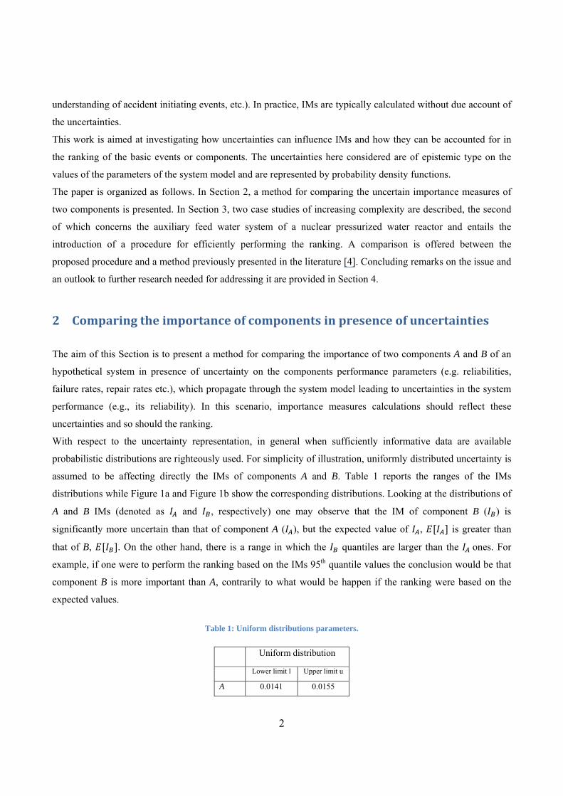
For further insights, it is of interest to relate the importance measures results obtained by the probabilistic
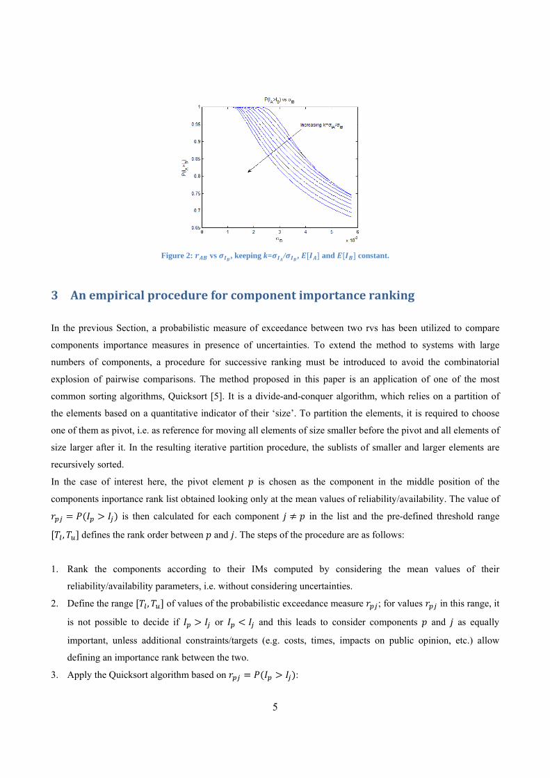
exceedance measure to the standard deviations of the IMs distributions, σ and σ . Figure 2
shows the variation of for increasing values of the standard deviation σ , keeping fixed the mean values of
IA and IB and the ratio σ / σ for different values of . In the extreme case of no uncertainties on the
knowledge of and (σ 0 and σ 0), component A is more important than B and thus 1.
Increasing the standard deviation σ (and thus also σ , keeping the ratio k constant), as expected 1 holds
as long as the pdfs of and do not overlap, i.e. and are uncertain quantities but it is not uncertain that
. The higher the ratio , the lower the set of points for which 1. Finally, as the overlapping
between pdfs increases decreases.
From the above considerations, it can be argued that uncertainties can affect the components importance rank
order and that reduction of uncertainties might be needed, in certain cases and when possible, for decreasing the
risk associated with the safety decision. To effectively drive the reduction of uncertainty, sensitivity analysis
may be used leading to the introduction of Uncertainty Importance Measures (UIMs) for identifying the
contribution of the epistemic uncertainty in the components performance parameters to the importance measures
uncertainty [6].
5
Figure 2: vs , keeping k= / , and constant.
3 An empirical procedure for component importance ranking
In the previous Section, a probabilistic measure of exceedance between two rvs has been utilized to compare
components importance measures in presence of uncertainties. To extend the method to systems with large
numbers of components, a procedure for successive ranking must be introduced to avoid the combinatorial
explosion of pairwise comparisons. The method proposed in this paper is an application of one of the most
common sorting algorithms, Quicksort [5]. It is a divide-and-conquer algorithm, which relies on a partition of
the elements based on a quantitative indicator of their ‘size’. To partition the elements, it is required to choose
one of them as pivot, i.e. as reference for moving all elements of size smaller before the pivot and all elements of
size larger after it. In the resulting iterative partition procedure, the sublists of smaller and larger elements are
recursively sorted.
In the case of interest here, the pivot element is chosen as the component in the middle position of the
components inportance rank list obtained looking only at the mean values of reliability/availability. The value of
is then calculated for each component in the list and the pre-defined threshold range
, defines the rank order between and . The steps of the procedure are as follows:
1. Rank the components according to their IMs computed by considering the mean values of their
reliability/availability parameters, i.e. without considering uncertainties.
2. Define the range , of values of the probabilistic exceedance measure ; for values in this range, it
is not possible to decide if or and this leads to consider components and as equally
important, unless additional constraints/targets (e.g. costs, times, impacts on public opinion, etc.) allow
defining an importance rank between the two.
3. Apply the Quicksort algorithm based on :
6
3.1. List the components in the rank order found in step 1.
3.2. Choose the middle element of the list (sublist) as pivot element, .
3.3. For each in the sublist compute the cdf, , of and evaluate 1 0 :
- If , then put j in the sublist of elements less important than .
- If , then put j in the sublist of elements more important than .
- If falls in , , then is equally important to .
3.4. Append the sublist of less important elements to the right of and the sublist of more important
elements to the left of
3.5. Recursively apply to each sublist steps 3.2- 3.4 until no sublist with more than one element exists.
More Details about the algorithm are given in Appendix 2.
4 Case studies To illustrate the method, two case studies of increasing complexity are provided:
1. a system made up of three components with uncertain failure rates lognormally distributed; this case allows
us to test the pairwise comparison criterion;
2. a complex system with all components in stand-by mode and periodically tested; the uncertain failure rates
are lognormally distributed; this case study allows us to explain in details the ranking procedure, with its
advantages and limitations.
As a term of comparison, the ranking procedure proposed in [4] has also been applied. This procedure follows
the same steps 1 and 2 above, whereas it differs in the steps 3 and 4, which are as follows:
3. Find the probability that each component 1, 2, … , occupies a specific position in the ranking. This is
achieved by repeating for 1, 2, … . , the following Monte Carlo sampling:
3.1. Sample a realization of the components’ failure rates , , … , .
3.2. Find the υ‐th IMs relative to the failure rates of 3.1.
3.3. Rank the components IMs.
3.4. The probability that component is in the rank position 1, 2,… , is given by the ratio
between the number of simulations with component resulting in position and the number of
samples M.
4. To rank the component:
7
4.1. List the components in the rank order found in step 1.
4.2. Choose the most important component as pivot , i.e. the component with largest probability of being
the most important.
4.3. Compute the measure of exceedance between the components and with 1, 2:
∑ ∑ (5)
where = rank of , and = rank of .
4.4. If , then leave component in the actual position; else, if then put the
component in position ; otherwise, if swap the rank orders of components and .
4.5. 1, repeat steps 4.1-4.3 until .
4.1 A threecomponent system
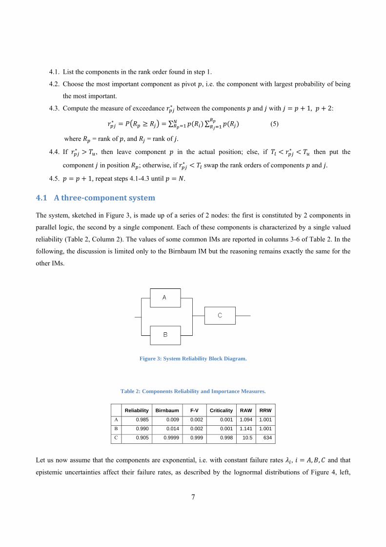
The system, sketched in Figure 3, is made up of a series of 2 nodes: the first is constituted by 2 components in
parallel logic, the second by a single component. Each of these components is characterized by a single valued
reliability (Table 2, Column 2). The values of some common IMs are reported in columns 3-6 of Table 2. In the
following, the discussion is limited only to the Birnbaum IM but the reasoning remains exactly the same for the
other IMs.
Figure 3: System Reliability Block Diagram.
Table 2: Components Reliability and Importance Measures.
Reliability Birnbaum F-V Criticality RAW RRW
A 0.985 0.009 0.002 0.001 1.094 1.001
B 0.990 0.014 0.002 0.001 1.141 1.001
C 0.905 0.9999 0.999 0.998 10.5 634
Let us now assume that the components are exponential, i.e. with constant failure rates , , , and that
epistemic uncertainties affect their failure rates, as described by the lognormal distributions of Figure 4, left,
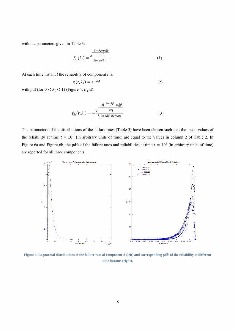
8
with the parameters given in Table 3:
· ·√ (1)
At each time instant t the reliability of component i is:
, (2)
with pdf (for 0 1) (Figure 4, right):
,
· ·√ (3)
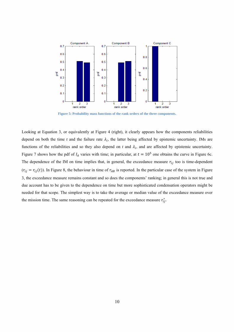
The parameters of the distributions of the failure rates (Table 3) have been chosen such that the mean values of
the reliability at time 10 (in arbitrary units of time) are equal to the values in column 2 of Table 2. In
Figure 6a and Figure 6b, the pdfs of the failure rates and reliabilities at time 10 (in arbitrary units of time)
are reported for all three components.
Figure 4: Lognormal distributions of the failure rate of component A (left) and corresponding pdfs of the reliability at different
time instants (right).
9
Table 3: Parameters of the lognormal distributions of the components failure rates.
Mean Variance
A 1.00e-007 5.00E-08
B 1.50e-007 5.00E-08
C 1.00e-006 5.00E-07
In spite of the simplicity of the considered system, finding the Birnbaum IM distributions by an analytical
approach is impracticable. To overcome this difficulty, Monte Carlo sampling has been applied. The resulting
distributions at the fixed time instant 10 are plotted in Figure 6c and Figure 6d. It can be noted that the
distribution of the IM of component C is displaced to larger values than that of components A and B, which
leaves no doubt that the most important component is C, as expected from the structure of the system and the
components reliability values. As for the ranking of A and B, one must compute the measure. The result
obtained by Monte Carlo sampling is 0.52, which with respect to 0.3 and 0.7 leads to conclude
that . Hence, the final components rank provided by the procedure here proposed sees C as the most
important element, followed by A and B equally important.
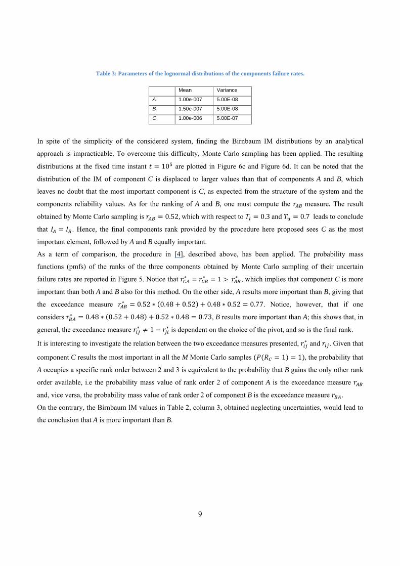
As a term of comparison, the procedure in [4], described above, has been applied. The probability mass
functions (pmfs) of the ranks of the three components obtained by Monte Carlo sampling of their uncertain
failure rates are reported in Figure 5. Notice that 1 , which implies that component C is more
important than both A and B also for this method. On the other side, A results more important than B, giving that
the exceedance measure 0.52 0.48 0.52 0.48 0.52 0.77. Notice, however, that if one
considers 0.48 0.52 0.48 0.52 0.48 0.73, B results more important than A; this shows that, in
general, the exceedance measure 1 is dependent on the choice of the pivot, and so is the final rank.
It is interesting to investigate the relation between the two exceedance measures presented, and . Given that
component C results the most important in all the M Monte Carlo samples 1 1 , the probability that
A occupies a specific rank order between 2 and 3 is equivalent to the probability that B gains the only other rank
order available, i.e the probability mass value of rank order 2 of component A is the exceedance measure
and, vice versa, the probability mass value of rank order 2 of component B is the exceedance measure .
On the contrary, the Birnbaum IM values in Table 2, column 3, obtained neglecting uncertainties, would lead to
the conclusion that A is more important than B.
10
Figure 5: Probability mass functions of the rank orders of the three components.
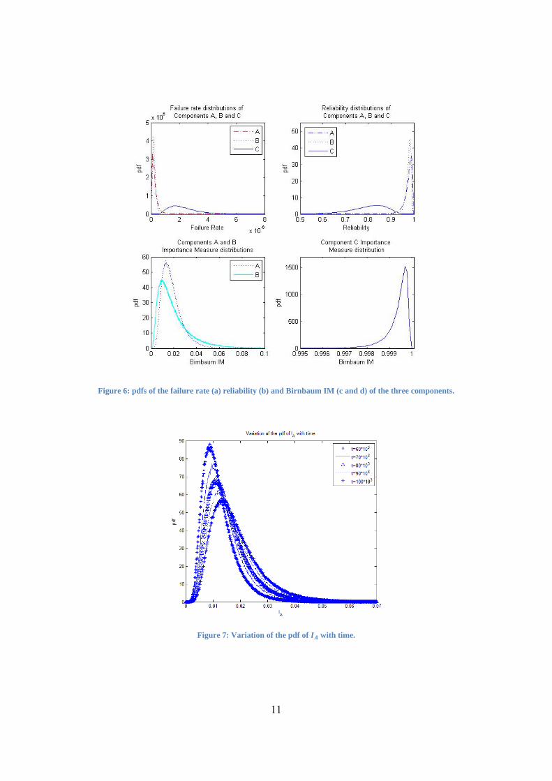
Looking at Equation 3, or equivalently at Figure 4 (right), it clearly appears how the components reliabilities
depend on both the time t and the failure rate , the latter being affected by epistemic uncertainty. IMs are
functions of the reliabilities and so they also depend on t and , and are affected by epistemic uncertainty.
Figure 7 shows how the pdf of varies with time; in particular, at 10 one obtains the curve in Figure 6c.
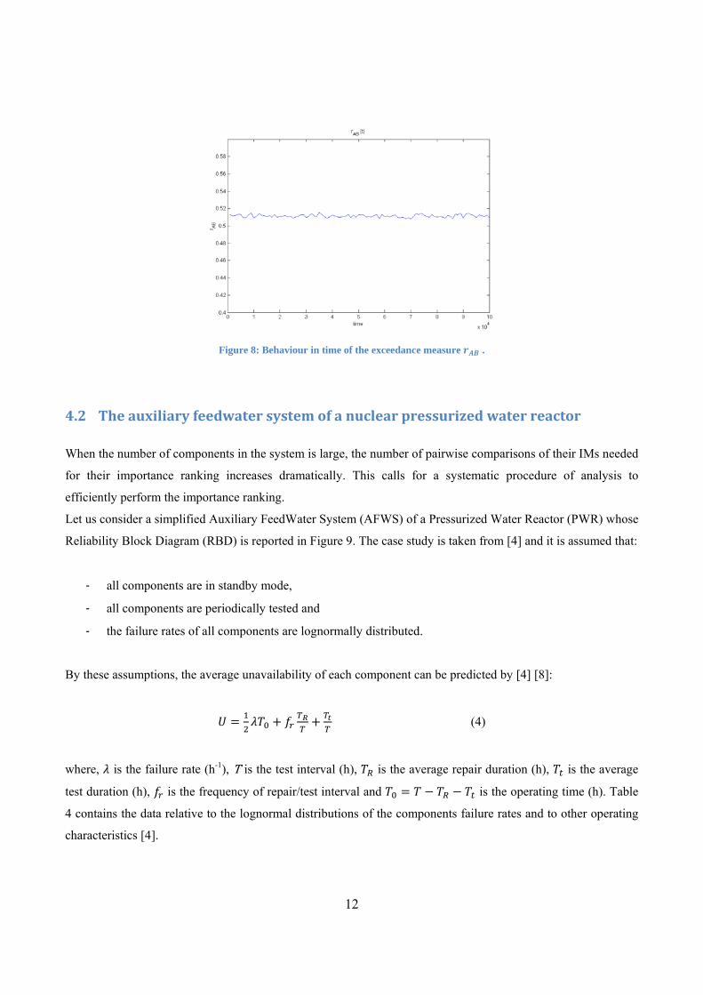
The dependence of the IM on time implies that, in general, the exceedance measure too is time-dependent
( ). In Figure 8, the behaviour in time of is reported. In the particular case of the system in Figure
3, the exceedance measure remains constant and so does the components’ ranking; in general this is not true and
due account has to be given to the dependence on time but more sophisticated condensation operators might be
needed for that scope. The simplest way is to take the average or median value of the exceedance measure over
the mission time. The same reasoning can be repeated for the exceedance measure .
11
Figure 6: pdfs of the failure rate (a) reliability (b) and Birnbaum IM (c and d) of the three components.
Figure 7: Variation of the pdf of with time.
12
Figure 8: Behaviour in time of the exceedance measure .
4.2 The auxiliary feedwater system of a nuclear pressurized water reactor
When the number of components in the system is large, the number of pairwise comparisons of their IMs needed
for their importance ranking increases dramatically. This calls for a systematic procedure of analysis to
efficiently perform the importance ranking.
Let us consider a simplified Auxiliary FeedWater System (AFWS) of a Pressurized Water Reactor (PWR) whose
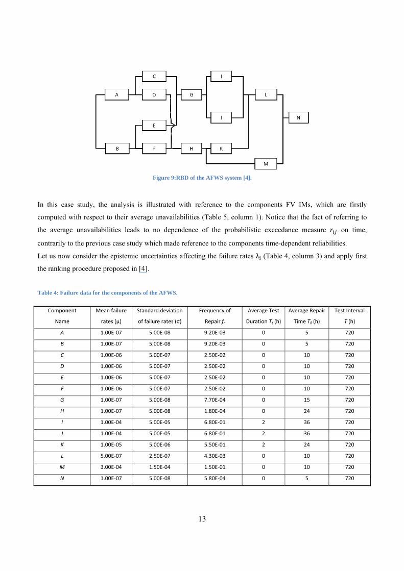
Reliability Block Diagram (RBD) is reported in Figure 9. The case study is taken from [4] and it is assumed that:
- all components are in standby mode,
- all components are periodically tested and
- the failure rates of all components are lognormally distributed.
By these assumptions, the average unavailability of each component can be predicted by [4] [8]:
(4)
where, is the failure rate (h-1), T is the test interval (h), is the average repair duration (h), is the average
test duration (h), is the frequency of repair/test interval and is the operating time (h). Table
4 contains the data relative to the lognormal distributions of the components failure rates and to other operating
characteristics [4].
13
Figure 9:RBD of the AFWS system [4].
In this case study, the analysis is illustrated with reference to the components FV IMs, which are firstly
computed with respect to their average unavailabilities (Table 5, column 1). Notice that the fact of referring to
the average unavailabilities leads to no dependence of the probabilistic exceedance measure on time,
contrarily to the previous case study which made reference to the components time-dependent reliabilities.
Let us now consider the epistemic uncertainties affecting the failure rates λ (Table 4, column 3) and apply first
the ranking procedure proposed in [4].
Table 4: Failure data for the components of the AFWS.
Component
Name
Mean failure
rates (µ)
Standard deviation
of failure rates (σ)
Frequency of
Repair fr
Average Test
Duration Tt (h)
Average Repair
Time TR (h)
Test Interval
T (h)
A 1.00E‐07 5.00E‐08 9.20E‐03 0 5 720
B 1.00E‐07 5.00E‐08 9.20E‐03 0 5 720
C 1.00E‐06 5.00E‐07 2.50E‐02 0 10 720
D 1.00E‐06 5.00E‐07 2.50E‐02 0 10 720
E 1.00E‐06 5.00E‐07 2.50E‐02 0 10 720
F 1.00E‐06 5.00E‐07 2.50E‐02 0 10 720
G 1.00E‐07 5.00E‐08 7.70E‐04 0 15 720
H 1.00E‐07 5.00E‐08 1.80E‐04 0 24 720
I 1.00E‐04 5.00E‐05 6.80E‐01 2 36 720
J 1.00E‐04 5.00E‐05 6.80E‐01 2 36 720
K 1.00E‐05 5.00E‐06 5.50E‐01 2 24 720
L 5.00E‐07 2.50E‐07 4.30E‐03 0 10 720
M 3.00E‐04 1.50E‐04 1.50E‐01 0 10 720
N 1.00E‐07 5.00E‐08 5.80E‐04 0 5 720
14
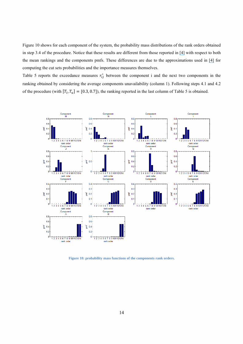
Figure 10 shows for each component of the system, the probability mass distributions of the rank orders obtained
in step 3.4 of the procedure. Notice that these results are different from those reported in [4] with respect to both
the mean rankings and the components pmfs. These differences are due to the approximations used in [4] for
computing the cut sets probabilities and the importance measures themselves.
Table 5 reports the exceedance measures between the component i and the next two components in the
ranking obtained by considering the average components unavailability (column 1). Following steps 4.1 and 4.2
of the procedure (with , 0.3, 0.7 ), the ranking reported in the last column of Table 5 is obtained.
Figure 10: probability mass functions of the components rank orders.
15
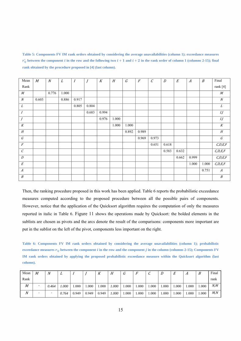
Table 5: Components FV IM rank orders obtained by considering the average unavailabilities (column 1); exceedance measures
between the component in the row and the following two and in the rank order of column 1 (columns 2-15); final
rank obtained by the procedure proposed in [4] (last column).
Then, the ranking procedure proposed in this work has been applied. Table 6 reports the probabilistic exceedance
measures computed according to the proposed procedure between all the possible pairs of components.
However, notice that the application of the Quicksort algorithm requires the computation of only the measures
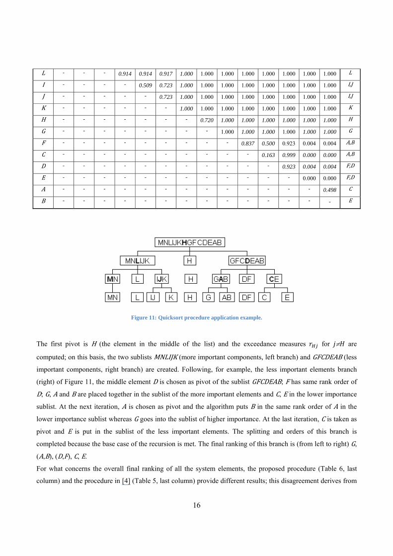
reported in italic in Table 6. Figure 11 shows the operations made by Quicksort: the bolded elements in the
sublists are chosen as pivots and the arcs denote the result of the comparisons: components more important are
put in the sublist on the left of the pivot, components less important on the right.
Table 6: Components FV IM rank orders obtained by considering the average unavailabilities (column 1); probabilistic
exceedance measures between the component in the row and the component in the column (columns 2-15); Components FV
IM rank orders obtained by applying the proposed probabilistic exceedance measure within the Quicksort algorithm (last
column).
Mean
Rank M N L I J K H G F C D E A B Final
rank
M - 0.464 1.000 1.000 1.000 1.000 1.000 1.000 1.000 1.000 1.000 1.000 1.000 1.000 N,M
N - - 0.764 0.949 0.949 0.949 1.000 1.000 1.000 1.000 1.000 1.000 1.000 1.000 M,N
Mean
Rank M N L I J K H G F C D E A B Final
rank [4]
M 0.776 1.000 M
N 0.603 0.886 0.917 N
L 0.805 0.804 L
I 0.683 0.994 I.J
J 0.976 1.000 I.J
K 1.000 1.000 K
H 0.892 0.989 H
G 0.969 0.973 G
F 0.651 0.618 C,D,E,F
C 0.583 0.632 C,D,E,F
D 0.662 0.999 C,D,E,F
E 1.000 1.000 C,D,E,F
A 0.751 A
B B
16
L - - - 0.914 0.914 0.917 1.000 1.000 1.000 1.000 1.000 1.000 1.000 1.000 L
I - - - - 0.509 0.723 1.000 1.000 1.000 1.000 1.000 1.000 1.000 1.000 I,J
J - - - - - 0.723 1.000 1.000 1.000 1.000 1.000 1.000 1.000 1.000 I,J
K - - - - - - 1.000 1.000 1.000 1.000 1.000 1.000 1.000 1.000 K
H - - - - - - - 0.720 1.000 1.000 1.000 1.000 1.000 1.000 H
G - - - - - - - - 1.000 1.000 1.000 1.000 1.000 1.000 G
F - - - - - - - - - 0.837 0.500 0.923 0.004 0.004 A,B
C - - - - - - - - - - 0.163 0.999 0.000 0.000 A,B
D - - - - - - - - - - - 0.923 0.004 0.004 F,D
E - - - - - - - - - - - - 0.000 0.000 F,D
A - - - - - - - - - - - - - 0.498 C
B - - - - - - - - - - - - - - E
Figure 11: Quicksort procedure application example.
The first pivot is H (the element in the middle of the list) and the exceedance measures for ≠ are
computed; on this basis, the two sublists MNLIJK (more important components, left branch) and GFCDEAB (less
important components, right branch) are created. Following, for example, the less important elements branch
(right) of Figure 11, the middle element D is chosen as pivot of the sublist GFCDEAB; F has same rank order of
D; G, A and B are placed together in the sublist of the more important elements and C, E in the lower importance
sublist. At the next iteration, A is chosen as pivot and the algorithm puts B in the same rank order of A in the
lower importance sublist whereas G goes into the sublist of higher importance. At the last iteration, C is taken as
pivot and E is put in the sublist of the less important elements. The splitting and orders of this branch is
completed because the base case of the recursion is met. The final ranking of this branch is (from left to right) G,
(A,B), (D,F), C, E.
For what concerns the overall final ranking of all the system elements, the proposed procedure (Table 6, last
column) and the procedure in [4] (Table 5, last column) provide different results; this disagreement derives from
17
the different numerical values of the exceedance measures (for example, 0.464 while 0.776).
These differences are due to the fact that, for any and , depends only on the importance measures of and
themselves whereas depends on the probability that a component occupies a specific order and thus also on
the importance measures of the other components of the system.
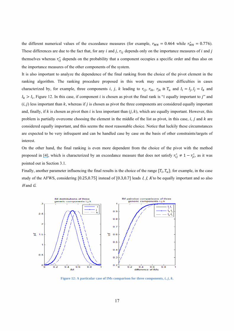
It is also important to analyze the dependence of the final ranking from the choice of the pivot element in the
ranking algorithm. The ranking procedure proposed in this work may encounter difficulties in cases
characterized by, for example, three components , , leading to , , and , and
, Figure 12. In this case, if component is chosen as pivot the final rank is “ equally important to ” and
( , ) less important than , whereas if is chosen as pivot the three components are considered equally important
and, finally, if is chosen as pivot then is less important than ( , ), which are equally important. However, this
problem is partially overcome choosing the element in the middle of the list as pivot, in this case, , and are
considered equally important, and this seems the most reasonable choice. Notice that luckily these circumstances
are expected to be very infrequent and can be handled case by case on the basis of other constraints/targets of
interest.
On the other hand, the final ranking is even more dependent from the choice of the pivot with the method
proposed in [4], which is characterized by an exceedance measure that does not satisfy 1 , as it was
pointed out in Section 3.1.
Finally, another parameter influencing the final results is the choice of the range , ; for example, in the case
study of the AFWS, considering 0.25,0.75 instead of 0.3,0.7 leads I, J, K to be equally important and so also
H and G.
Figure 12: A particular case of IMs comparison for three components, , , .
18
5 Conclusions
In this work, a procedure is proposed for ranking system components in order of importance when in presence of
epistemic uncertainties affecting the components reliability and availability parameters. The procedure is based
on the definition of a probabilistic exceedance measure that permits to compare the importance of two
components and on the application of the Quicksort algorithm for effectively performing the pairwise
comparisons needed to sort all the system components on the basis of their importance measures. The
application of the proposed procedure to two case studies has shown the relevance of accounting for
uncertainties in the computation of IMs: the ranking of the components’ importances obtained neglecting the
uncertainties can be different from that obtained by considering them.
Compared to another approach proposed in the literature, the procedure here presented seems to overcome some
limitations through a more satisfactory definition of the exceedance measure and a greater robustness of the final
rank from the choice of the pivot element in the sorting algorithm.
Acknowledgments
The work is funded by CESI RICERCA S.p.A. The views expressed in this paper are solely those of the authors.
References
[1] Birnbaum, Z.W. (1969). On the importance of different components in a multi component system.
Multivariate analysis II, New York, Academic Press.
[2] Youngblood, R.W. (2001). Risk significance and safety significance. Reliability Engineering and System
Safety; 73; 121-136.
[3] Apostolakis, G.E. (1990). The concept of probability in safety assessments of technological systems,
Science, 250; 1359-1364.
[4] Modarres, M. (2006). Risk Analysis in Engineering: Probabilistic Techniques, Tools and Trends, CRC
Press.
[5] Hoare, C.A. (1962). Quicksort, Computer Journal, 5; 10-15.
[6] Borgonovo, E. (2006) Measuring uncertainty importance: investigation and comparison of alternative
approaches, Risk Analysis, Vol. 26, N. 5; 1349-1361.
[7] K. Durga Rao, H.S. Kushwaha, A.K. Verma, A. Srividya (2007): Quantification of epistemic and aleatory
uncertainties in level 1 probabilistic safety assessment, Reliability Engineering & System Safety; 92; 947-956.
[8] Zio, E. (2006). An introduction to the basics of reliability and risk analysis, Singapore, World Scientific
Publishing.
19
[9] Knuth, D. (1997). The Art of Computer Programming, Volume 3: Sorting and Searching, Third Edition.
Addison-Wesley.
[10] Rausand, M. & Hoyland, A. (2004). System Reliability Theory, Wiley.
[11] Birolini, A. (2004). Reliability Engineering. Springer.
[12] Schneeweiss, W.G. (2001). Reliability Modeling, LiLoLe-Verlag.
Appendix 1
Given a generic uniform rv x≈U(a,b), its moment generating function (mgf) is given by:
)()(
absees
sasb
−−
=φ
The rv r=IA-IB is the convolution of two uniformly distributed random variables and in particular:
IA≈U(aIA,bIA);
-IB≈U(-bIB,-aIB);
The mgf of r is given by:
)()()(
)()(
BB
BIBI
AA
AIAI
II
bsas
II
sasb
r absee
absees
−−
⋅−−
=−−
φ
)()()( 2
)()()()(
BBAA
BIAIBIAIBIAIBIAI
IIII
basbbsaasabs
r ababseeees
−⋅−+−−
=−−−−
φ
For what concerns the inverse transformation, it could be noted that the mgf of r can be regarded as the algebraic
sum of functions linearly increasing/decreasing with the same slope. So the pdf and cdf of r are given by:
⎪⎪⎪⎪
⎩
⎪⎪⎪⎪
⎨
⎧
−≤≤−−⋅−
−−
−≤≤−−
−≤≤−−⋅−
−+
=
BABA
BBAA
BA
BABA
BB
BABA
BBAA
AB
IIIIIIII
II
IIIIII
IIIIIIII
II
r
abraaabab
rab
aarbbab
bbrbaabab
abr
rf
)()(
)(1
)()(
)(
20
⎪⎪⎪⎪⎪
⎩
⎪⎪⎪⎪⎪
⎨
⎧
−≤≤−−⋅−
−−
−
−≤≤−−⋅
⋅−⋅−+−
−≤≤−−⋅−⋅
+−
=
BABA
BBAA
BA
BABA
BB
BAA
BABA
BBAA
AB
IIIIIIII
II
IIIIII
III
IIIIIIII
II
r
abraaabab
rab
aarbbab
raba
bbrbaabab
rab
rF
)()(2
)(
1
)(2)22(
1
)()(2)(
)(
2
2
Appendix 2
A common method of simplification of a complex problem is to divide the problem into sub-problems of the
same type: this technique in computer programming is called ‘divide and conquer’. Quicksort algorithm applies
such technique and sorts groups of elements by dividing their list (ordered array) into two sub-lists. In its simpler
version the steps are:
• List the elements in an array ordered according to a given size parameter.
• Pick an element, called a pivot, from the list.
• Reorder the list so that all elements which are smaller than the pivot come before the pivot and all
elements larger than the pivot come after it (equal values can go either way).
• After this partitioning, the pivot is in its final position. This is called the partition operation.
• Recursively sort the sub-list of smaller elements and the sub-list of larger elements, following the steps
above.
The base case of the recursion (i.e. the stopping condition where the sorting function will not call itself anymore)
are lists of size zero or one. In a simple pseudocode format, the algorithm used in this work might be delineated
as follows:
function quicksort(array)
var list less, greater, equal
if length(array) ≤ 1 then return array
pivot:=the middle element of array
put pivot into equal
for each x in array
21
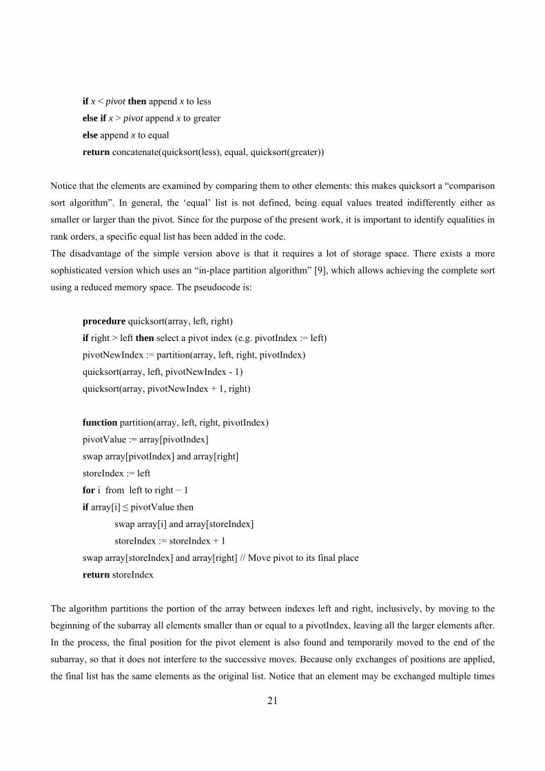
if x < pivot then append x to less
else if x > pivot append x to greater
else append x to equal
return concatenate(quicksort(less), equal, quicksort(greater))
Notice that the elements are examined by comparing them to other elements: this makes quicksort a “comparison
sort algorithm”. In general, the ‘equal’ list is not defined, being equal values treated indifferently either as
smaller or larger than the pivot. Since for the purpose of the present work, it is important to identify equalities in
rank orders, a specific equal list has been added in the code.
The disadvantage of the simple version above is that it requires a lot of storage space. There exists a more
sophisticated version which uses an “in-place partition algorithm” [9], which allows achieving the complete sort
using a reduced memory space. The pseudocode is:
procedure quicksort(array, left, right)
if right > left then select a pivot index (e.g. pivotIndex := left)
pivotNewIndex := partition(array, left, right, pivotIndex)
quicksort(array, left, pivotNewIndex - 1)
quicksort(array, pivotNewIndex + 1, right)
function partition(array, left, right, pivotIndex)
pivotValue := array[pivotIndex]
swap array[pivotIndex] and array[right]
storeIndex := left
for i from left to right − 1
if array[i] ≤ pivotValue then
swap array[i] and array[storeIndex]
storeIndex := storeIndex + 1
swap array[storeIndex] and array[right] // Move pivot to its final place
return storeIndex
The algorithm partitions the portion of the array between indexes left and right, inclusively, by moving to the
beginning of the subarray all elements smaller than or equal to a pivotIndex, leaving all the larger elements after.
In the process, the final position for the pivot element is also found and temporarily moved to the end of the
subarray, so that it does not interfere to the successive moves. Because only exchanges of positions are applied,
the final list has the same elements as the original list. Notice that an element may be exchanged multiple times

22
before reaching its final place. This kind of algorithm might be useful when a very large number of components
has to be sorted.