A GLOBAL HUMAN WALKING MODEL WITH REAL-TIME KINEMATIC PERSONIFICATION

Ronan Boulic, Nadia Magnenat-Thalmann, Daniel Thalmann

Abstract

This paper presents a human walking model built from experimental data based on a wide range ofnormalized velocities. The model is structured in two levels. At a first level, global spatial and temporalcharacteristics (normalized length and step duration) are generated. At the second level, a set ofparameterized trajectories produce both the position of the body in the space and the internal bodyconfiguration . This is performed for a standard structure and an average configuration of the human body.

The experimental context corresponding to the model is extended by allowing a continuous variation ofglobal spatial and temporal parameters according to the motion rendition expected by the animator. Themodel is based on a simple kinematic approach designed to keep the intrinsic dynamic characteristics of theexperimental model. Such an approach also allows a personification of the walking action in an interactivereal-time context in most cases. A correction automata of such motion is then proposed.

Keywords: animation, Biomechanic, walk, gait, inverse kinematics.

1. Introduction

Research in Computer Animation tends to be more and more oriented towards animation of complex scenesinvolving human beings conscious of their environment (Thalmann et al. 1988). This type of animation ismultidisciplinary because it has to integrate some aspects and methods specific to animation, mechanics,robotics, physiology and artificial intelligence.

In order to create naturalistic human motion, it is essential to take into account the geometric, physical andbehavioral aspects. No system based on only one of these aspects can give good results.

To improve the natural aspect of motion, several authors (Isaacs and Cohen 1987; Wilhelms 1987; Girardand Maciejewski 1985; Armstrong and Green 1985; Arnaldi et al 1989) have introduced dynamic laws,but generally for simple characters with a few joints because of the important CPU costs of such models.

In fact, the use of a dynamic model requires switching from a problem of specifying positional jointparameters to one of specifying applied forces and torques. This new parameter space is not easier tomanipulate. The introduction of inverse dynamics for dynamically processing predefined trajectories doesnot solve the problem of how to find the natural trajectory for a specified task. This goal is partially reached by using criterion optimizing methods (energy-based constraints). Combined with other criteria integratingthe physiological limitations of joints, dynamic models have shown to be appropriate for the specification ofcertain movements: leg balance in walking (Bruderlin and Calvert 1989), hand motion from one location toanother (Girard 1989).

However, when the motion involves an interaction with the environment (e.g. contact force in a walkingaction) the expression of such criteria is not trivial and the problem is still open. Moreover, the integrationof a personification of motion may satisfy the animator but may be incompatible from a physical point ofview. Likewise, results obtained by solving equations may lead to stereotype movements for persons with

the same anatomic configuration. Another drawback of dynamic models is the excessive cost in terms ofCPU time which prevents the appreciation of the motion in real-time. This is a major restriction for thedesign of a motion, especially walking which involves expressive information of behavioral, social andcultural nature.

In this context, we propose a method based on a mathematical parameterization coming from biomechanicalexperimental data. The main idea of this method is to take advantage of the intrinsic dynamics of the studiedmotion and extend its application context to a wider range but producing results which are realistic andinteresting for the animator. From a taxonomy point of view such a method can be considered as anextension of the traditional rotoscopy method. We are interested in the human walking because of itsfundamental importance which also means that numerous studies in biomechanics are available. The maindirections of our method are applicable to other classes of human movements more or less complex thanwalking. The lack of experimental data could seem a serious drawback for these other fields of applications;however, Biomechanics has also been involved in other classes of human movement as rehabilitation orsports. Finally, in image analysis, there are research project in automatic determination of temporalevolution of a motion - at the joint level - from a series of 2D images (Ferrigno and Pedotti 1985 , TEMISproject IRISA Rennes).

2. Human walking

By definition, walking is a form of locomotion in which the body's center of gravity moves alternately onthe right side and the left side. At all times at least one foot is in contact with the floor and during a briefphase both feet are in contact with this floor.

2.1 Previous researches

Descriptions of biped gait, and especially human gait, has been extensively studied in Biomechanics (Inmanet al. 1980; Murray et al. 1964; Saunders et al. 1953; Lamoreux 1971). In robotics, much has been writtenconcerning biomechanics for conception of artificial walking systems (Gurfinkel and Fomin 1974; Hemamiand Farnsworth 1977; Miura and Shimoyama 1984; McMahon 1984). Several dance notations have alsobeen proposed (Eshkol and Wachman 1958; Hutchinson 1970) and walking has been described using thesenotations (Badler and Smoliar 1979). Finally, several authors (Calvert and Chapman 1978; Zeltzer 1982;Magnenat-Thalmann and Thalmann 1987; Girard and Maciejewski 1985; Girard 1987; Bruderlin andCalvert 1989; Zeltzer 1988 ) have developed systems for generating computer-animated walking sequences.

2.2 Definitions

As walking is a cyclic activity, we only study the portion of motion between two successive contacts of theleft heel with the floor. Fig.1 shows the temporal structure of the walking cycle with the main time andduration information. Fig.2 presents the spatial structure of the same cycle.

DdsDds

50%0% 100%

left footright foot

timeDuration of cycle

Duration of support Duration of balance

HSTO HS

HSTOTO

Fig. 1. Temporal structure of the walking cycleDc: Duration of cycle; HS: Heel Strike ; TO: Toe Off; Ds: Duration of support (duration of contact withthe floor); Db: Duration of balance (duration of non-contact with the floor); Dds: duration of doublesupport

step length

cycle length

cycle width

Foot aperture

Fig. 2. Spatial structure of the walking cycle

3. The proposed model

3.1 Introduction

The proposed model is intended for producing for any point in time the values of the spatial, temporal andjoint parameters of the free walking human being with average characteristics (Kreighbaum and Barthels1985). All spatial values of the model are normalized by the fundamental characteristic of the walk: theheight of the thigh (noted Ht). This is the length between the flexing axis of the thigh and the foot sole, asshown in Fig.3. The average value is 53% of the total height of the human being (Kreighbaum and Barthels1985)

zy x

z

H Ht s

Fig. 3. Definition of the body coordinate system and the initial position

α > π α<π

3ο 3ο

3ο

Fig. 4. Stretched and rest positions of the knee

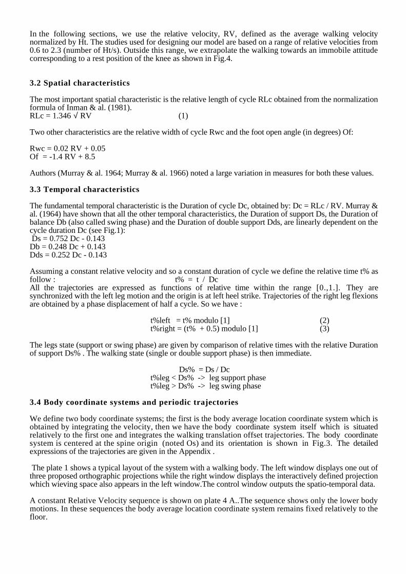
In the following sections, we use the relative velocity, RV, defined as the average walking velocitynormalized by Ht. The studies used for designing our model are based on a range of relative velocities from0.6 to 2.3 (number of Ht/s). Outside this range, we extrapolate the walking towards an immobile attitudecorresponding to a rest position of the knee as shown in Fig.4.

3.2 Spatial characteristics

The most important spatial characteristic is the relative length of cycle RLc obtained from the normalizationformula of Inman & al. (1981).RLc = 1.346 √ RV (1)

Two other characteristics are the relative width of cycle Rwc and the foot open angle (in degrees) Of:

Rwc = 0.02 RV + 0.05Of = -1.4 RV + 8.5

Authors (Murray & al. 1964; Murray & al. 1966) noted a large variation in measures for both these values.

3.3 Temporal characteristics

The fundamental temporal characteristic is the Duration of cycle Dc, obtained by: Dc = RLc / RV. Murray &al. (1964) have shown that all the other temporal characteristics, the Duration of support Ds, the Duration ofbalance Db (also called swing phase) and the Duration of double support Dds, are linearly dependent on thecycle duration Dc (see Fig.1): Ds = 0.752 Dc - 0.143Db = 0.248 Dc + 0.143Dds = 0.252 Dc - 0.143

Assuming a constant relative velocity and so a constant duration of cycle we define the relative time t% asfollow : t% = t / DcAll the trajectories are expressed as functions of relative time within the range [0.,1.]. They aresynchronized with the left leg motion and the origin is at left heel strike. Trajectories of the right leg flexionsare obtained by a phase displacement of half a cycle. So we have :

t%left = t% modulo [1] (2)t%right = (t% + 0.5) modulo [1] (3)

The legs state (support or swing phase) are given by comparison of relative times with the relative Durationof support Ds% . The walking state (single or double support phase) is then immediate.

Ds% = Ds / Dct%leg < Ds% -> leg support phaset%leg > Ds% -> leg swing phase

3.4 Body coordinate systems and periodic trajectories

We define two body coordinate systems; the first is the body average location coordinate system which isobtained by integrating the velocity, then we have the body coordinate system itself which is situatedrelatively to the first one and integrates the walking translation offset trajectories. The body coordinatesystem is centered at the spine origin (noted Os) and its orientation is shown in Fig.3. The detailedexpressions of the trajectories are given in the Appendix .

The plate 1 shows a typical layout of the system with a walking body. The left window displays one out ofthree proposed orthographic projections while the right window displays the interactively defined projectionwhich wieving space also appears in the left window.The control window outputs the spatio-temporal data.

A constant Relative Velocity sequence is shown on plate 4 A..The sequence shows only the lower bodymotions. In these sequences the body average location coordinate system remains fixed relatively to thefloor.

3.5 Discussion

We have built a model which may be used at two levels:

. first at a global level in order to generate the average temporal and spatial characteristics (normalized).

. then at the trajectory level in order to describe at each time the position of the body in space and itsinternal configuration.

Before going further, let us introduce the concept of virtual floor. This is the plane supporting the body atthe initial position (see Fig.3 ). Its height is defined by the initial height of the origin of the spine noted Hs.Its average value is about 58% of the total size of the human being (Dreyfuss 1966). It will be useful toconsider and to manipulate a virtual floor coordinate system linked to the body average location coordinatesystem.

As the model comes from the synthesis of a large number of experimental data and not from solving motionequations, it is logical to obtain a rather realistic approximation which does not correspond exactly to thesupport constraint of the virtual floor. This problem may be overcome by modifying the leg flexing usingan inverse kinematics method. This method is described in the section prediction/correction. Such a methodallows a decisive extension of the model to fill the expressive needs of the animator.

relative cycle time

average covered dist.

priorities and spatial - temporal coherence

normalizedtrajectories

walking cycleautomaton

DcDs, Db, DdsDs%RLc

RV

RVt

RLc

globalnormalizedcharacteristics

∆t

t%leftt%right

Rwc , Of

fc

Rd

Walking motor

temporal characteristics

spatial characteristics

Fig. 5. Walking motor

4. Extension of the application field of the model

4.1 Spatial and temporal parameters

When strictly applied, a relative velocity, assumed to be constant, completely determines a free walking fora flat floor with a straight direction. However, it is clear that such a context is too limited for an animatorwho would like to recreate variable situations in space and time. Consequently, we propose to extend thisstrict context by the following points:

A provide as entry points the three variables linked by the formula RV=RLc/Dc with the following priorities (see Fig.5):

- if the relative velocity is specified, it determines the two other variables- if only the relative cycle length varies, the cycle duration is fixed and the relative velocity is adjusted- if only the cycle duration varies, the relative cycle length is fixed and the relative velocity is adjusted- if only the relative cycle length and the cycle duration vary, the relative velocity is adjusted

The three last possibilities cannot be considered as a free walking; the obtained gait is a decelerated oraccelerated free gait. The gait is realistic in the neighborhood of the characteristic (1). Otherwise it willprovide a larger parameter space allowing the designer to guarantee a global spatial or temporalconstraint. In particular, it will be possible to freeze any motion phase with an infinite cycle duration (infact, we work with the frequency fc expressed in number of cycles /second which is zero in this case).

B allow a continuous variation of the previous entry points while maintaining the coherence of walking. This allows adaptation to an environment which varies fast (e.g. displacement in a crowd)

C project the covered distance by the body at each time onto an independently defined path. RV(t), the instantaneous relative velocity is integrated to provide the average relative covered distance (noted Rd) This distance, multiplied by the Ht of the considered human being and projected onto the average path, produces the body average location coordinate system. To obtain the exact body coordinate system we have to add the instantaneous translation offset dependent on RV and t%.

4.2 Personification

At the present stage, our walk motor may respond to a wide range of qualitative needs of the animator fromthree point of views: the general walk function (RV), the attitude (RLc) and the animation (Dc or fc).However the personification of the motion is intrinsically average and therefore it is necessary to introducean extra level of individuality.Our approach to this problem is rather simple but available independently for each instantaneouscharacteristic (body location and configuration):

personified motion = α . reference motion + β

A random perturbation mechanism is also proposed independently for α and β by specifying the maximalamplitude and the smoothing level of a reference noise.

All the parameters of personification are continuously modifiable and the visual result is synchronized onthe clock model in order to correctly evaluate the design of the personified motion. The continuous variationof the spatial-temporal parameters also allows the designer to appreciate the characterization within the fullrange of relative velocities.Of course, such a freedom for the animator may produce gaits which do not correspond to any free walk:this is our goal. It should be noted that the introduction of the personification does not modify the spatialand temporal coherence (t%, RV) of the initial model. The assumption of the small modifications may beinvalidated by the animator's creativity. This suggests that several adaptation methods have to be proposed,which will be discussed in the section on prediction/correction.

An illustration of personification is given by plate 2 (whole body) and plate 4 sequence B (lower body)where the motions were amplified interactively by the animator to produce this kind of running movement.

4.3 Primary adaptation

Behavior range may become wider by constraining the motion in order to respect some kind of support forthe feet and by extension the shoes.

Five levels of constraint may be introduced. In increasing order:

1. the support height stays at the virtual floor level

2. the height and the orientation of the support basis are constrained to the virtual floor

3. the support position stays fixed in the world coordinate system of the corresponding virtual floor.

4. the position and the orientation of the support basis are constrained in the world coordinatesystem of the corresponding virtual floor.

5. the support location is conformed to the world floor (this constraint is under research in order tocoordinate walk and vision).

The application of these constraints is driven by the global characteristics of the model. In the case of a verypersonified gait, the spatial characteristics are generally false and make obsolete the use of constraints. Wepropose to fix the value of a personified velocity PV based on the value of a personified lenght of cyclePLc. These two values are characterized by Ht and more generally by the given skeleton and its supportattributes.

bodycoordinate

systemsituation andindividualized

configuration for t%=0

support referencePLc

PHsHs

body average location coordinate system

virtual floor level

Fig. 6. Personification and primary adaptation

The value PLc is roughly evaluated as follows (see Fig. 6):

- current personification data are used to derive the situation and the configuration of the human being forthe time t%=0.

- PLc is then approximated by twice the distance along the displacement axis (xbody) between the left andright support references.

We have PV= PLc / Dc and the personified average covered distance Pd is obtained by integrating PV.

Similarly, a personified height of spine can be used to tune the maximum amplitude of the body verticaloffset in order to meet a support on the virtual floor. This value PHs is approximated by the distancebetween the body average location coordinate system and the support reference which starts (see Fig.6).This primary adaptation guarantees a global spatial and temporal coherence sufficient to apply theconstraints. Moreover, we provide two methodologies for following paths. In fact either the animator doesnot care about the trajectory followed by the body coordinate system or he does not care about thecoincidence of the virtual floor with a particular world floor. For us, a path is a 3D trajectory associatedwith a vector defining the vertical direction when it is necessary to define it. A path is in private mode whenit is followed by the body average location coordinate system. In this case, the height of the virtual floordoes not necessarily coincide with a reference linked to the world according to the variations ofcharacterization (Ht, skeleton) or personification (see Fig.7). A path is in public mode when it is followed

by the virtual floor coordinate system. A support, linked to the path, is guaranteed for any human being orpersonification (see Fig.8).

world coordinate system

path coordinatesystem

virtual floorcoordinate

system

body average location coordinate system

Fig. 7. A path in private mode

world coordinate system

path coordinatesystem

virtual floorcoordinate

system

body average location coordinate system

Fig. 8. A path in public mode

5. Functional diagram

The functional diagram (shown in Fig.9) is based on two blocks of prediction-correction which drive theprocessing of walking at the current time. It also uses a module producing the current values of the highlevel parameters. This module is strictly limited to predefined or interactive directives. It does not adaptthem for a specific task like the adaptation of path velocity in order to lay the foot at specific locations. Thisis under research but ,when the animator uses real-time tools, he interacts continuously with the system at ahigher level and may control himself these adaptative behaviors.

5.1 Prediction

Prediction provides several levels of sophistication in the design – without constraints – of gaits. Theanimator may and should work by stepwise refinements.

For the complete case, the prediction process is as follows:

From the current state of the system : This state meets the specified constraints. Otherwise, amethod of initial correction should modify it. The state at the time t+∆t now has to be built from thecurrent value of the high level parameters RV, RLc and fc .

High Level Parameters Handling

Walk motor

Personification with primary adaptation

Pathtracking

Transitionevaluation

support <-> swing

PREDICTION

LEGCORRECTION

incrementalcorrection

Adjustement

condition on the maximal coach joint increment

Evaluation of the residual error on theconstraints

success

failure

Globalcharacteristics

trajectories

Supportcharacteristics

t∆t

Globalcharacteristics

per

son

ifie

d t

raje

ctor

y

incr

emen

t on

per

son

ifie

d t

raje

ctor

y

Con

stra

ints

Pat

h t

rack

ing

Per

son

ific

atio

nS

pat

ial-

tem

por

al

Success

accepted

Dec

reas

ing

∆t

Corrected prediction

accepted

denied

denied

high initial error on the

constraints

Actualization of state and current time eventual increase of ∆t

Correction methods automata

Prediction update

Body / world situation

PV , Pd , PHs

Figure 9 Functional diagram

Walk motor : As the global parameters vary continuously we have to maintain the coherence of thewalking trajectories of both legs. This was achieved by a frequency modulation of the initial model. Inthe initial context we had : ∆t% = ∆t / Dc

For the continuous variation case we assume dt% = dt / Dc(t)

so t% = ∫ fc(t) dt

wich gives , in the restrictive case of (modulated) free walking :t% = 0.495 √ RV(t)3Otherwise a numerical integration is used.

Expressions (2) and (3) still hold to produce t%right and t%left .

An example of an increasing Relative Velocity sequence is shown in plate 4 C .

Personification : If required the primary adaptation is done wich produces the current velocity PV(t) andby integration the average covered distance Pd(t).

Path tracking : The projection of this distance onto the desired path is immediate.In fact, The path ismodelled using cardinal splines which have the advantage of passing through the control points. It istransformed before the tracking phase in a sequence of line segments using an adaptative samplingalgorithm (Koparkar and Mudur 1983). The incremental process for making correspondence betweenthe curvilinear abscissa with the distance Pd(t) is then trivial. We obtain the position of the bodyaverage location coordinate system or the position of the virtual floor coordinate system according to theselected mode. The tangent to the curve provides the forward direction. An extra vector (normal to theforward direction) for the vertical locates the set consisting of the body and the virtual floor relative tothe path.

Transition evaluation : The last proposed module for prediction determines the areas of potentialpersonification support. Rather than to restrict ourselves to the strictly defined phases defined in 3.3,which impose constraints on start and end of phases that are hard to maintain, we prefer derive thesevalues from the current personification. This requires the specification of one support out of the fourproposed: heel, base (linked to the ankle), toe and extremity (linked to the toe). A support request iscreated as soon as the reference point associated with a support passes under the virtual floor. Theserequests have a priority which is proportional to the measured divergence.

5.2 Correction

The coach concept

Even with the primary adaptation the personified trajectories may induce large deviations for the desiredconstraints. Inverse kinematics methods can deal with such a problem by means of adaptative time step oreven a correction loop at constant time until the constraints are met. But the more the personified motion iscorrected the more it looses its intrinsic dynamics.

That's why we introduce the concept of coach wich retains the personified data and drives the correctionmethod. In our context of walking this concept is applied only to the legs for the correction method to workon two simple kinematic chains. At a first stage the coach is used to update the prediction as follow. Let ∆abe the joint angle deviation between the coach and the current corrected configuration (for each leg) :

- If ∆a is low the prediction includes all the personified motion including the coach.- If ∆a is important the prediction integrates the personified motion of the body situation and pelvis rotation while the leg keeps the current corrected configuration.

The coach concept is illustrated in the plate 3 where we are in a low level constraint context.This means that a virtual floor level constraint is applied only when there is a request of support from one of

the support reference points. In this case no constraint is applied to the front leg because it is just beforeheel strike. So the front leg and its coach still coïncide.On the other hand the back leg does not coïncide with its coach because the corrections due to the constrainthas been configuring it differently since the first support request. The next prediction will include thecurrent corrected configuration because of the large ∆a deviation with its coach. The correction will bedriven by the tracking of the coach kinematics while meeting the constraints.

Our approach to inverse kinematics

The general form of the solution provided by inverse kinematics is often used in robotics (Espiau andBoulic 1985) and Computer Animation (Girard 1989):

∆θ = J+∆x + (I-J+J) z

where:

∆θ is the joint space solution of the inverse kinematic problemJ is the Jacobian matrix associated with the main taskJ+ is the unique pseudo inverse of J and provides the minimum norm solution to achieve the main task∆x describes the main task to achieve in cartesian spacez describes the secondary task in joint space which is partially achieved on the null space of the main task.

This means that the second term of the solution does not affect the achievement of the main task (∀z); z is

chosen in order to minimize a cost function c such as z = -µ ∇c (µ>0)

The application of this technique to walking has consisted of a strictly tracking of spatial and temporaltrajectories considered as main tasks assigned to feet (or other end effectors) as defined by Girard (1989) orZeltzer and Sims (1988). An eventual secondary task of optimization of the joint limits may complete thesolution (Girard and Maciejewski 1985). The major drawback of this approach is essentially animpersonnal style of walking.

We have chosen a more qualitative specification based on the walk motor:

Our main task is to respect the support of the floor on support request and to switch to a simple coach tracking when no support is required.

Our secondary task is to keep track of the coach kinematics ; this integrates two configurations increments :

-The first is proportionnal to the configuration deviation ∆a in order to catch up the coach configuration after the end of the support phase

-The second is equal to the coach variation in order to retain its intrinsic dynamics

The interest of such an approach is to keep the natural dynamics of the initial model. It requires a lowdimensional constraint space to maximize the dimension of the Null space on which the secondary task isperformed.The main difficulty is to provide a smooth switching when the main task commute between support andno_support phases. This is currently under investigation and we are evaluating an automata managing thedifferent correction methods (fig 10). The main idea is to define an intermediate correction method , calledthe mixed-correction, which is the "missing link" between inverse and direct kinematics methods. In thismethod we progressively insert the mapped secondary task into the main task while the former constraintsprogressively disappear due to the beginning of the swing phase:

∆θ = J+(∆x + k.Jz) + (I-J+J) z with 0 ≤ k ≤ 1

So when the resulting main task reduces to the full mapped secondary task it is equivalent to a directkinematics method :∆θ = J+Jz + (I-J+J) z = z

In this way we fullfil the continuous switching requirement .

The initial correction method is just a correction loop at constant time wich switches to the other correctionmethods as soon as the initial constraints are met.

The implementation has been carried out in the C language using the Silicon Graphics IRIS 4D workstation.

INITIAL CORRECTION

TRACKING CORRECTION

MIXED CORRECTION

COPY OF COACH

(PRS : Prédiction Request of Support )

PRSPRS

end of PRS

end of PRS

no PRS

Stick to Support

far

near

INVERSE KINEMATICS

DIRECT KINEMATICS

Coach Kinematics Tracking

Stick Constraint

CONSTRAINED CORRECTION

Stick ConstraintCoach static Tracking

FromInitialConfiguration

end of Stick toSupport

INVERSE KINEMATICS

INVERSE KINEMATICS

Coach Kinematics Tracking

Coach Kinematics Tracking

Stick Constraint and Coach Kinematics Tracking

Figure 10. Correction Methods Automata

6. Conclusion

We have proposed an important extension of a walking model based on experimental data. The animatormay use a wide range of stepwise refinements for the design of real-time gaits. Its major advantage is toallow a qualitative and continuous design of a gait using the dynamic feeling of an experimental model.

Current research direction is to evaluate extensively our correction automata in order to extend this approachto the correction of any other type of predefined motions (recorded , model-based, key-framed). Anothertrend is to conceive a continuous control loop of the high level parameters for the next step locationhandling. This would be used for obstacle avoidance or displacement in a discrete foot location space(examples : white parts of a checker board, japanese garden etc...).

7. Acknowledgments

The authors are grateful to Dominique Boisvert and Denis Rambaud for their great help for the imageproduction interface. We also wishes to thank Olivier Renault for video support and Arghyro Paouri for theray-casting sequences production.The research was supported by the Fonds National Suisse pour la Recherche Scientifique, the NaturalSciences and Engineering Council of Canada, the FCAR foundation and the Institut National de laRecherche en Informatique et Automatique (France).

8. References

Armstrong WW, Green MW (1985) Dynamics for Animation of Characters with Deformable Surfaces in:N.Magnenat-Thalmann, D.Thalmann (Eds) Computer-generated Images, Springer, pp.209-229.

Arnaldi B, Dumont G, Hégron G, Magnenat-Thalmann N, Thalmann D (1989) Animation Control UsingDynamics, in: State of the Art in Computer Animation, Springer, Tokyo

Badler NI, Smoliar SW (1979) Digital Representation of Human Movement, ACM Computing Surveys,March issue, pp.19-38.

Bruderlin A, Calvert TW (1989) Goal Directed, Dynamic Animation of Human Walking, Proc.SIGGRAPH '89, Computer Graphics, Vol. 23, No3

Calvert TW, Chapman J (1978) Notation of Movement with Computer Assistance, Proc. ACM AnnualConf., Vol.2, 1978, pp.731-736

Dreyfuss H (1966) The Measure of Man, 2nd edition, Withney library of design, New York.Eshkol N, Wachmann A (1958) Movement Notation, Weidenfeld and Nicolson, LondonEspiau B, Boulic R (1985) Collision Avoidance for Redundant Robots with Proximity Sensors, Proc. 3rd

International Symposium of Robotic Research, Gouvieux, France, Octobre 1985Ferrigno G, Pedotti A (1985) ELITE : a Digital dedicated hardware system for movement analysis via real-

time TV signal processing IEEE Trans. on Biomedical Engeneering BME-32(11)943-950Girard M (1987) Interactive Design of 3D Computer-animated Legged Animal Motion, IEEE Computer

Graphics and Applications, Vol.7, No6, pp.39-51Girard M (1989) Constrained Optimization of Articulated Animal Movements in Computer Animation,

M.I.T. Workshop on Mechanics, Control, and Animation of Articulated FiguresGirard M, Maciejewski AA (1985) Computational Modeling for Computer Generation of Legged Figures,

Proc. SIGGRAPH '85, Computer Graphics, Vol. 19, No3, pp.263-270Gurfinkel VS, Fomin SV (1974) Biomechanical Principles of Constructing Artificial Walking Systems, in:

Theory and Practice of Robots and Manipulators, Vol.1, Springer, NY, pp.133-141Hemami H, Farnsworth RL (1977) Postural and Gait Stability of a Planar Five Link Biped by Simulation,

IEEE Trans. on Automatic Control, AC-22, No3, pp.452-458.Hutchinson A (1970) Labanotation, Theatre Books, NYInman VT, Ralston HJ, Todd F (1981) Human Walking, Baltimore, Williams & WilkinsIsaacs PM, Cohen MF (1987) Controlling Dynamic Simulation with Kinematic Constraints, Bahvior

Functions and Inverse Dynamics, SIGGRAPH'87, Computer Graphics, Vol.21, No4, pp.215-224Koparkar PA and Mudur SP (1983) A New Class of Algorithms for the Processing of Parametric Curves,

Computer-aided Design, Vol.15, No1, pp.41-45Kreighbaum E, Barthels KMB (1985) Biomechanics, a qualitative approach, 2nd edition, Burgess

publishing Company, Minneapolis, Minn.Lamoreux LW (1971) Kinematic Measurements in the Study of Human Walking, Bulletin of Prosthetics

Research, Vol.BPR 10, No15Magnenat-Thalmann N, Thalmann D (1987) The Direction of Synthetic Actors in the film Rendez-vous à

Montréal, IEEE Computer Graphics and Applications, Vol. 7, No 12. pp.9-19.McMahon T (1984) Mechanics of Locomotion, Intern. Journ. of Robotics Research, Vol.3, No2, pp.4-28.Miura H, Shimoyama I (1984) Dynamic Walk of a Biped, International Journal of Robotics, Vol.3, No2,

pp.60-74.Murray MP, Drought AB, Kory RC (1964) Walking Patterns of Normal Men, Journal of Bone Joint

Surgery, Vol.46A, No2, pp.335-360Murray P, Kory RC, Clarkson BH, Sepic SB (1966) Comparison of Free and Fast Speed Walking Patterns

of Normal Men, American Journal of Physical Medecine, Vol.45, No 1, pp.8-24Murray P (1967) Gait as a total pattern of movement, American Journal of Physical Medecine, Vol.46, No

1, pp.290-333Saunders JB, Inman VT, Eberhart (1953) The Major Determinants in Normal and Pathological Gait,

Journal of Bone Joint Surgery, Vol.35A, pp.543-558Thalmann D, Magnenat-Thalmann N, Wyvill B, Zeltzer D, SIGGRAPH '88 Tutorial Notes on Synthetic

Actors: the Impact of A.I. and Robotics on Animation.Wilhelms J (1987) Using Dynamic Analysis for Realistic Animation of Articulated Bodies, IEEE Computer

Graphics and Applications, Vol.7, No 6, pp.12-27Zarrugh MY, Radclifh CW (1979) Computer generation of Human Gait Kinematics, Journal of

Biomechanics, Vol.12, pp.99-111Zeltzer D, Sims K (1989) A Figure Editor and Gait Controller to Task Level Animation in: Thalmann D,

Magnenat-Thalmann N, Wyvill B, Zeltzer D, SIGGRAPH '88 Tutorial Notes on Synthetic Actors: theImpact of A.I. and Robotics on Animation.

Appendix Trajectory models are based on the studies of Murray (1964,1966,1967) and Zarrugh(1979).

(All the rotationnal amplitudes are expressed in degrees.)

A: Periodic trajectories situating the body

Location of the body in the space: three translation trajectory coordinates situate the body relatively to theaverage position it has while moving with the velocity RV.

Vertical translation: the height of Os decreases for completing the step. The amplitude of this decreasegrows with RV. this function express a vertical offset from the current height ofspine Hs.

amplitude: Av = 0.015 RV

expression: -Av + Av sin 2π (2 t%-0.35)

Lateral translation: Os oscillates laterally in order to ensure the weight transfer from one leg to the other leg. The amplitude is almost always constant.

amplitude: for RV>0.5 Al = -0.032for RV<0.5 Al = -0.128 RV2 + 0.128 RV

expression: Al sin 2π (t% - 0.1)

a positive value expresses a displacement on the left side of the human being

Translation forward/backward: (lead/delay) For an average velocity RV, the body has in fact acceleration and deceleration phases which correspond to the advance to the new

step then the stabilization on the new leg. This effect decreases when RV grows because of the smoothing effect due to the kinetic energy.

amplitude: for RV>0.5 Aa = -0.021 for RV<0.5 Aa = -0.084 RV2 + 0.084 RV

phase displacement: φa = 0.625 - Ds%

expression: Aa sin 2π (2t%+2φa)

a positive value states for an advance relatively to the average position

B: Periodic trajectories of internal rotations of the pelvis

Rotation forward/backward: this flexing movement of the back relatively to the pelvis is done justbefore each step to move the center of gravity of the body in order to help the forwardmotion of the leg.

amplitude: for RV>0.5 A1 = 2 for RV<0.5 A1 = -8 RV2 + 8 RV

expression: -A1 + A1 sin 2π (2 t%-0.1)

Rotation left/right: the pelvis falls on the side of the swinging leg

amplitude: A2 = 1.66 RV

expression: 0 ≤t%< 0.15 -A2 + A2 cos 2π (10/3 t%)

0.15 ≤t%< 0.5 -A2 - A2 cos 2π (10/7 (t% - 0.15))

0.5 ≤t%< 0.65 A2 - A2 cos 2π (10/3 (t% - 0.5))

0.65 ≤t%< 1 A2 + A2 cos 2π (10/7 (t% - 0.65))

Torsion rotation: the pelvis may rotate relatively to the spine in order to perform the step more easily

amplitude: A3 = 4 RV

expression: -A3 cos 2π t%

a negative value expresses a pelvis torsion towards the left leg

These three trajectories strongly depend on the individual human being .

C : Periodic trajectories of the leg flexing/extension

The truly walking trajectories are the trajectories of flexing/extension at the thigh, the knee, the ankle andthe toe. These trajectories are very similar from one human being to another one on an experimental rangeof relative velocities.

Trajectories of flexing/extension are modelled using cubic splines passing through control points located atthe extremities of the trajectories. The coordinates of these points are noted (t%i,y i) for the control point i.The modelling of the variations of these few points in function of RV is sufficient to rebuild the expectedtrajectory.We use two of the basic Hermit splines :

h1(s) = 2s3-3s2+1 (decreasing step)h2(s)=-2s3+3s2 (increasing step)

An increasing portion of trajectory f(t%,RV) with t% between t%i-1 and t%i is expressed as follows:

f(t%,RV) = yi + (yi-yi-1) h2[(t%-t%i-1)/(t%i-t%i-1)]

where the values of t%j and yj depend on RV.

The study of the variation of control points in function of RV is performed on the following three ranges:

range gaits

A 0. ≤RV< 0.5 starts from the immobile attitude to reach a slow gaitB 0.5 ≤RV< 1.3 slow gait almost constantC 1.3 ≤RV< 3. significant evolution of the gait

B.1 Flexing at the hip

The first figure indicates the three necessary control points. The variation of their coordinates aresummarized in the second figure.

0 10 20 30 40 50 60 70 80 90 100

0

-20

+20

+40

2

31

positionstandingstretched

t%

Flexing at the hip

A B C0

-0.1

0,1

0.5

0.9

1

t%1

t%2

t%3

A B C0

10

20

30

-10

-20

y1

y3

y2

25

-15

30

31degrees

RV

RV

Variations of the coordinates of the control point in function of the relative velocity

B.2 Flexing at the knee

The first figure indicates the four necessary control points. The variation of their coordinates aresummarized in the second figure.

0

+20

+40

+60

+80

1

2

3

4

stop

0 10 20 30 40 50 60 70 80 90 100

t%positionstandingstretchedFlexing at the knee

A B C0

0.971

t%1

t%2

t%3

t%4

0.75 0.70

0.4

0.17 0.12

A B C00

y3

y1

y4y2

36

25

6570

degrees

0

10

20

30

40

50

60

70

RV

RVVariations of the coordinates of the control point in function of the relative velocity

B.3 Flexing at the ankle

The first figure indicates the five necessary control points. The variation of their coordinates aresummarized in the second figure.

0

-20

+20

1

2

3

4

5

0 10 20 30 40 50 60 70 80 90 100

positionstandingstretched

t%

flexing at the ankle

A B C0

1

t%1

t%2

t%3

t%4

0.85

0,5

0.08 Toe on

0,4

Toe off

t%5

Ds%

A B Cy3

y1 , y 5

y2

y4

0

10

-10

-20

8 52

-3

-18-14

-20 -28

RV

RV

degrees

Variations of the coordinates of the control point in function of the relative velocity

The closer a joint is to the floor, the more complex is its trajectory and the more it tends to be modifiedbecause of the variation of the floor surface. Consequently, it is useless to model the trajectory of the anklewith great accuracy.. In addition we have derived the toe flexing from the other flexing angles in order tomaintain the toe horizontal during the stance phase.

D : Periodic trajectories of the upper-body

D.1 Motion of the Thorax

As noted by Murray (1967) the torsion of the thorax in a direction opposite to that of the pelvis contributesto the smothness of translation by providing counterbalancing restraints against excessive motion of theentire torso. As the pelvis motion this one also strongly depends on each human being.

The first figure indicates the four necessary control points. The variation of their coordinates aresummarized in the second figure (relative time coordinates remain constant with Relative Velocity).

0 10 20 30 40 50 60 70 80 90 100

23

1t%

0

3

- 3

4

cotédroit

cotégauche

- 3

0

3

AB

C RV

4.54

- 4-4.5

y1

y4

y3

y2

Degrees

Thorax torsion amplitude coordinate variations

In addition to thorax torsion we have completed the thorax motion by a side oscillation in opposition phasewith the torsion and with an amplitude.divided by a constant factor. This produces a balancing of the thoraxon the side of the swinging leg.

D.2 Flexing at the shoulder : the arm is in phase with the opposite foot.

amplitude AS = 9.88 RV

expression REST_VALUE - AS / 2. - AS cos 2 π t%

A positive value expresses a front swinging motion.A rest value of three degrees beyond the vertical is due to the momentum of the forearm and the hand.

D.3 Flexing at the elbow : the forearm motion is similar to the arm with some delay and a quicker backward motion.

The first figure indicates the three necessary control points. The variation of their coordinates aresummarized in the second figure.

0 10 20 30 40 50 60 70 80 90 100

0

2

31

t%

Elbow limit

20

40

60

rest value3

Flexing at the elbow

A B CRV

y1

y3

y2

0

20

40

60

1720

70

44

degrees

RVA B C

1

0.05

0.55

0.9 0.8

t%1

t%2

t%3

0.50.51

3 148

6

118

Variations of the coordinates of the control points in function of the relative velocity

Plate 1: A typical layout of the system.

Plate 2: An attitude from a personified motion

Plate 3: The coach concept

Plate 4: Gait sequences (with constant time intervals)

Ronan Boulic is a research assistant in the Computer GraphicsLab at the Swiss Federal Institute of Technology in Lausanne,Switzerland. His current research interests are 3D computeranimation related to perception-action control loops and real-timeman-machine interaction. He received his engineer diploma from theNational Institute of Applied Sciences (INSA) of Rennes in 1983and Computer Sciences Doctorate from the University of Rennes(France) in 1986. He spent one year as a visiting research associateat the MIRALab Laboratory of the Graduate Business School of theUniversity of Montreal. address: EPFL-LIG CH 1015 Lausanne, SwitzerlandE-mail: boulic@ligsg2.epfl.ch

Nadia Magnenat Thalmann is currently full Professor ofComputer Science at the University of Geneva, Switzerland. Aformer member of the Council of Science and Technology of theGovernment of Quebec and of the Council of Science andTechnology of the Canadian Broadcasting Corporation, she also hasserved on a variety of government advisory boards and programcommittees. She has received several awards, including the 1985Communications Award from the Government of Quebec. In May1987, she was nominated woman of the year in sciences by theMontreal community. Dr. Magnenat Thalmann received a BS inpsychology, an MS in biochemistry, and a Ph.D in quantumchemistry and computer graphics from the University of Geneva.Her previous appointments include the University Laval in Quebec,the Graduate Business school of the University of Montreal inCanada. She has written and edited several books and researchpapers in image synthesis and computer animation and wascodirector of the computer-generated films Dream Flight, Eglantine,Rendez-vous à Montréal and Galaxy Sweetheart. She served aschairperson of the Canadian Graphics Interface 85 Conference inMontreal and the CG International 88 conference.address: MIRALab, CUI

University of Geneva12 rue du LacCH 1207 Geneva, Switzerland

E-mail: thalmann@uni2a.unige.ch

Daniel Thalmann is currently full Professor and Director of theComputer Graphics Laboratory at the Swiss Federal Institute ofTechnology in Lausanne, Switzerland. Since 1977, he wasProfessor at the University of Montreal and codirector of theMIRALab research laboratory. He received his diploma in nuclearphysics and Ph.D in Computer Science from the University ofGeneva. He is member of the editorial board of the Visual Computerand cochairs the EUROGRAPHICS Working Group on ComputerSimulation and Animation. He was director of the Canadian Man-Machine Communications Society and is a member of the ComputerSociety of the IEEE, ACM, SIGGRAPH, and the ComputerGraphics Society. Daniel Thalmann's research interests include 3Dcomputer animation, image synthesis, and scientific visualization.He has published more than 60 papers in this areas and is coauthorof several books including: Computer Animation: Theory andPractice and Image Synthesis: Theory and Practice. He is alsocodirector of several computer-generated films: Dream Flight,Eglantine, Rendez-vous à Montréal, Galaxy Sweetheart.address: Computer Graphics Lab

Swiss federal Institute of TechnologyCH 1015 Lausanne, Switzerland

E-mail: thalmann@elma.epfl.ch