
A comparison of Data Stores for the Online Feature ... - kth .diva
211
IN DEGREE PROJECT COMPUTER SCIENCE AND ENGINEERING, SECOND CYCLE, 30 CREDITS , STOCKHOLM SWEDEN 2021 A comparison of Data Stores for the Online Feature Store Component A comparison between NDB and Aerospike ALEXANDER VOLMINGER KTH ROYAL INSTITUTE OF TECHNOLOGY SCHOOL OF ELECTRICAL ENGINEERING AND COMPUTER SCIENCE
-
Upload
khangminh22 -
Category
Documents
-
view
1 -
download
0
Transcript of A comparison of Data Stores for the Online Feature ... - kth .diva

IN DEGREE PROJECT COMPUTER SCIENCE AND ENGINEERING,SECOND CYCLE, 30 CREDITS
, STOCKHOLM SWEDEN 2021
A comparison of Data Stores for the Online Feature Store Component
A comparison between NDB and Aerospike
ALEXANDER VOLMINGER
KTH ROYAL INSTITUTE OF TECHNOLOGYSCHOOL OF ELECTRICAL ENGINEERING AND COMPUTER SCIENCE

A comparison of Data Storesfor the Online Feature StoreComponentA comparison between NDB and Aerospike
ALEXANDER VOLMINGER
Civilingenjör DatateknikDate: April 25, 2021Supervisor: Jim DowlingExaminer: Stefano MarkidisSchool of Electrical Engineering and Computer ScienceHost company: Spotify ABSwedish title: En jämförelse av datalagringssystem för andvändingsom Online Feature StoreSwedish subtitle: En jämförelse mellan NDB och Aerospike

A comparison of Data Stores for the Online Feature StoreComponent / En jämförelse av datalagringssystem förandvänding som Online Feature Store
© 2021 Alexander Volminger

Abstract | i
Abstract
This thesis aimed to investigate what Data Stores would fit to be implementedas an Online Feature Store. This is a component in the Machine Learninginfrastructure that needs to be able to handle low latency Reads at highthroughput with high availability. The thesis evaluated the Data Stores withreal feature workloads from Spotify’s Search system. First an investigation wasmade to find suitable storage systems. NDB and Aerospike were selectedbecause of their state-of-the-art performance together with their suitablefunctionality. These were then implemented as the Online Feature Store bybatch Reading the feature data through a Java program and by using GoogleDataflow to input data to the Data Stores.
For 1 client NDB achieved about 35% higher batch Read throughput witharound 30% lower P99 latency than Aerospike. For 8 clients NDB got 20%higher batch Read throughput, with a varying P99 latency different comparedto Aerospike. But in a 8 node setup NDB achieved on average 35% lowerlatency. Aerospike achieved 50% faster Write speeds when writing feature datato the Data Stores. Both Data Stores’ Read performance was found to sufferupon Writing to the data store at the same time as Reading, with the P99 Readlatency increasing around 30% for both Data Stores. It was concluded thatboth Data Stores would work as an Online Feature Store. But NDB achievedbetter Read performance, which is one of the most important factors for thistype of Feature Store.
Keywords
Feature Stores, Data Stores, NDB, Aerospike, NoSQL, Online Feature Stores

ii | Sammanfattning
Sammanfattning
Den här uppsatsen undersökte vilka datalagringssystem som passar föratt implementeras som en Online Feature Store. Detta är en komponent imaskininlärningsinfrastrukturen som måste hantera snabba läsningar med höggenomströmning och hög tillgänglighet. Uppsatsen studerade detta genom attevaluera datalagringssystem med riktig feature data från Spotifys söksystem.En utredning gjordes först för att hitta lovande datalagringssystem för dennauppgift. NDB och Aerospike blev valda på grund av deras topp prestandaoch passande funktionalitet. Dessa implementerades sedan som en OnlineFeature Store genom att batch-läsa feature datan med hjälp av ett Java programsamt genom att använda Google Dataflow för att lägga in feature datan idatalagringssystemen.
För 1 klient fick NDB runt 35% bättre genomströmning av feature data jämförtmed Aerospike för batch läsningar, med ungefär 30% lägre P99 latens. För 8klienter fick runt 20% högre genomströmning av feature data med en P99 latenssom var mer varierande. Men klustren med 8 noder fick NDB i genomsnitt35% lägre latens. Aerospike var 50% snabbare på att skriva feature datantill datalagringssystemet. Båda systemen led dock av sämre läsprestanda närskrivningar skedde till dem samtidigt. P99 läs-latensen gick då upp runt30% för båda datalagringssystemen. Sammanfattningsvis funkade båda avde undersökta datalagringssystem som en Online Feature Store. Men NDBhade bättre läsprestanda, vilket är en av de mest viktigaste faktorerna för denhär typen av Feature Store.
Nyckelord
Feature Stores, Datalagringsystem, NDB, Aerospike, NoSQL, Online FeatureStores

Acknowledgments | iii
Acknowledgments
I would like to thank my supervisor at KTH, Prof. Jim Dowling, for overseeingthe thesis work, helping me structure the benchmark and for sharing hisextensive knowledge about Feature Stores. I would also like thank all theamazing people at Spotify whom I have been speaking with throughout thethesis. Special thanks to my supervisor at Spotify, Daniel Lazarovski, for thetechnical guidance and general support. But also to Anders Nyman for thesupport throughout the thesis and the rest of the Search team at Spotify. LastlyI want to thank Mikael Ronström at Logical Clocks for all the help with NDBand thoughts in general about the thesis.
Stockholm, March 2021Alexander Volminger

iv | CONTENTS
Contents
1 Introduction 11.1 Problem Description . . . . . . . . . . . . . . . . . . . . . . 21.2 Purpose . . . . . . . . . . . . . . . . . . . . . . . . . . . . . 21.3 Research Question . . . . . . . . . . . . . . . . . . . . . . . 21.4 Research Methodology . . . . . . . . . . . . . . . . . . . . . 31.5 Delimitations . . . . . . . . . . . . . . . . . . . . . . . . . . 31.6 Structure of the thesis . . . . . . . . . . . . . . . . . . . . . . 4
2 Background 52.1 Feature Data Stores . . . . . . . . . . . . . . . . . . . . . . . 52.2 Data Models . . . . . . . . . . . . . . . . . . . . . . . . . . . 7
2.2.1 RDBMS . . . . . . . . . . . . . . . . . . . . . . . . 72.2.2 NoSQL . . . . . . . . . . . . . . . . . . . . . . . . . 8
2.3 Distributed Systems . . . . . . . . . . . . . . . . . . . . . . . 102.3.1 Skewed Data and Hot Spots . . . . . . . . . . . . . . 112.3.2 Partitioning/Sharding . . . . . . . . . . . . . . . . . . 11
2.4 Client-Server Data Stores . . . . . . . . . . . . . . . . . . . . 122.4.1 NDB Cluster . . . . . . . . . . . . . . . . . . . . . . 122.4.2 Aerospike . . . . . . . . . . . . . . . . . . . . . . . . 132.4.3 Redis . . . . . . . . . . . . . . . . . . . . . . . . . . 142.4.4 Dynamo . . . . . . . . . . . . . . . . . . . . . . . . . 152.4.5 Riak . . . . . . . . . . . . . . . . . . . . . . . . . . . 162.4.6 BigTable . . . . . . . . . . . . . . . . . . . . . . . . 162.4.7 HBase . . . . . . . . . . . . . . . . . . . . . . . . . . 172.4.8 Cassandra . . . . . . . . . . . . . . . . . . . . . . . . 172.4.9 Netflix’s Hollow . . . . . . . . . . . . . . . . . . . . 18
2.5 Previous Benchmarks . . . . . . . . . . . . . . . . . . . . . . 192.5.1 Redis, HBase & Cassandra . . . . . . . . . . . . . . . 20

CONTENTS | v
2.5.2 PostgreSQL, Redis & Aerospike . . . . . . . . . . . . 202.5.3 YCSB . . . . . . . . . . . . . . . . . . . . . . . . . . 222.5.4 Jepsen . . . . . . . . . . . . . . . . . . . . . . . . . . 23
2.6 Choice of Data Stores . . . . . . . . . . . . . . . . . . . . . . 23
3 Experimental Procedure 253.1 Data . . . . . . . . . . . . . . . . . . . . . . . . . . . . . . . 25
3.1.1 Feature Requests . . . . . . . . . . . . . . . . . . . . 253.1.2 Feature Data . . . . . . . . . . . . . . . . . . . . . . 26
3.2 Experimental design . . . . . . . . . . . . . . . . . . . . . . 263.2.1 Workloads . . . . . . . . . . . . . . . . . . . . . . . 263.2.2 Test Environment . . . . . . . . . . . . . . . . . . . . 273.2.3 Data Store Cluster Setups . . . . . . . . . . . . . . . 283.2.4 Measurements . . . . . . . . . . . . . . . . . . . . . 29
4 Implementation 314.1 Read Benchmark . . . . . . . . . . . . . . . . . . . . . . . . 32
4.1.1 NDB . . . . . . . . . . . . . . . . . . . . . . . . . . 324.1.2 Aerospike . . . . . . . . . . . . . . . . . . . . . . . . 33
4.2 Write Program . . . . . . . . . . . . . . . . . . . . . . . . . 344.2.1 NDB . . . . . . . . . . . . . . . . . . . . . . . . . . 354.2.2 Aerospike . . . . . . . . . . . . . . . . . . . . . . . . 35
4.3 Cluster Configurations . . . . . . . . . . . . . . . . . . . . . 364.3.1 NDB . . . . . . . . . . . . . . . . . . . . . . . . . . 364.3.2 Aerospike . . . . . . . . . . . . . . . . . . . . . . . . 37
5 Results and Discussion 385.1 Read Benchmark . . . . . . . . . . . . . . . . . . . . . . . . 38
5.1.1 One Client . . . . . . . . . . . . . . . . . . . . . . . 385.1.2 Several Clients . . . . . . . . . . . . . . . . . . . . . 43
5.2 Write Program . . . . . . . . . . . . . . . . . . . . . . . . . 465.2.1 Memory Usage . . . . . . . . . . . . . . . . . . . . . 49
5.3 Write & Read Benchmark . . . . . . . . . . . . . . . . . . . . 49
6 Conclusions and Future Work 536.1 Conclusions . . . . . . . . . . . . . . . . . . . . . . . . . . . 536.2 Sustainability and Ethics . . . . . . . . . . . . . . . . . . . . 556.3 Future work . . . . . . . . . . . . . . . . . . . . . . . . . . . 55
References 56

vi | CONTENTS
A Benchmark Tables 62A.1 Read Benchmark . . . . . . . . . . . . . . . . . . . . . . . . 62
A.1.1 NDB . . . . . . . . . . . . . . . . . . . . . . . . . . 62A.1.2 Aerospike . . . . . . . . . . . . . . . . . . . . . . . . 65
A.2 Read & Write Benchmark . . . . . . . . . . . . . . . . . . . . 67A.2.1 NDB . . . . . . . . . . . . . . . . . . . . . . . . . . 67A.2.2 Aerospike . . . . . . . . . . . . . . . . . . . . . . . . 69
B Cluster Configurations 71B.1 NDB Configuration . . . . . . . . . . . . . . . . . . . . . . . 71B.2 Aerospike Configuration . . . . . . . . . . . . . . . . . . . . 75
C Availability Zones 78C.1 NDB . . . . . . . . . . . . . . . . . . . . . . . . . . . . . . . 78C.2 Aerospike . . . . . . . . . . . . . . . . . . . . . . . . . . . . 79
D Hardware Utilization 80D.1 Read Benchmark . . . . . . . . . . . . . . . . . . . . . . . . 80
D.1.1 1 Client, 6 Nodes & 1 Thread . . . . . . . . . . . . . 80D.1.2 1 Client, 6 Nodes & 2 Threads . . . . . . . . . . . . . 84D.1.3 1 Client, 6 Nodes & 4 Threads . . . . . . . . . . . . . 88D.1.4 1 Client, 6 Nodes & 8 Threads . . . . . . . . . . . . . 92D.1.5 1 Client, 6 Nodes & 16 Threads . . . . . . . . . . . . 96D.1.6 1 Client, 6 Nodes & 32 Threads . . . . . . . . . . . . 100D.1.7 2 Clients, 6 Nodes & 16 Threads . . . . . . . . . . . . 104D.1.8 2 Clients, 6 Nodes & 32 Threads . . . . . . . . . . . . 108D.1.9 4 Clients, 6 Nodes & 16 Threads . . . . . . . . . . . . 110D.1.10 8 Clients, 6 Nodes & 16 Threads . . . . . . . . . . . . 114D.1.11 1 Client, 8 Nodes & 1 Thread . . . . . . . . . . . . . 120D.1.12 1 Client, 8 Nodes & 2 Threads . . . . . . . . . . . . . 124D.1.13 1 Client, 8 Nodes & 4 Threads . . . . . . . . . . . . . 128D.1.14 1 Client, 8 Nodes & 8 Threads . . . . . . . . . . . . . 132D.1.15 1 Client, 8 Nodes & 16 Threads . . . . . . . . . . . . 136D.1.16 1 Client, 8 Nodes & 32 Threads . . . . . . . . . . . . 140D.1.17 2 Clients, 8 Nodes & 16 Threads . . . . . . . . . . . . 144D.1.18 4 Clients, 8 Nodes & 16 Threads . . . . . . . . . . . . 148D.1.19 8 Clients, 8 Nodes & 16 Threads . . . . . . . . . . . . 152
D.2 Write Program . . . . . . . . . . . . . . . . . . . . . . . . . 157D.2.1 6 Nodes & 128 workers . . . . . . . . . . . . . . . . . 157D.2.2 6 Nodes & 256 workers . . . . . . . . . . . . . . . . . 158

CONTENTS | vii
D.2.3 6 Nodes & 512 workers . . . . . . . . . . . . . . . . . 162D.2.4 8 Nodes & 256 Workers . . . . . . . . . . . . . . . . 166D.2.5 8 Nodes & 512 Workers . . . . . . . . . . . . . . . . 169
D.3 Write & Read Benchmark . . . . . . . . . . . . . . . . . . . . 173D.3.1 6 Nodes & 256 Workers . . . . . . . . . . . . . . . . 173D.3.2 6 Nodes & 512 Workers . . . . . . . . . . . . . . . . 179D.3.3 8 Nodes & 256 Workers . . . . . . . . . . . . . . . . 185D.3.4 8 Nodes & 512 Workers . . . . . . . . . . . . . . . . 190

viii | LIST OF FIGURES
List of Figures
4.1 Shows how the Feature Store fits into the larger picture. . . . . 31
5.1 Throughput of 1 client in 6 and 8 node setup . . . . . . . . . . 395.2 Latency of 1 client in 6 node setup . . . . . . . . . . . . . . . 405.3 Latency of 1 client in 8 node setup . . . . . . . . . . . . . . . 415.4 Client’s peak CPU in percentage for the 8 node setups . . . . . 425.5 Average throughput of the clients in both 6 and 8 node setup
of NDB and Aerospike . . . . . . . . . . . . . . . . . . . . . 435.6 Average latency of the clients in 6 node setup for NDB and
Aerospike . . . . . . . . . . . . . . . . . . . . . . . . . . . . 445.7 Average latency of the clients in 8 node setup for NDB and
Aerospike . . . . . . . . . . . . . . . . . . . . . . . . . . . . 445.8 CPU peak utilization in the Data Store in percentages . . . . . 455.9 Data Store Cluster Nodes peak CPU in percentages . . . . . . 475.10 Average batch Read throughput of 8 clients while the Write
load was applied with 256 and 512 workers . . . . . . . . . . 495.11 Average batch Read latency of the clients in both node setups
while Write load was applied . . . . . . . . . . . . . . . . . . 505.12 The Data Stores Node’s peak CPU in percentages . . . . . . . 51

LIST OF TABLES | ix
List of Tables
2.1 Data Store solutions for online feature serving in Feature Stores[1] . . . . . . . . . . . . . . . . . . . . . . . . . . . . . . . . 7
3.1 GCP hardware resources used by each node type . . . . . . . 28
5.1 NDB’s Total Write Time . . . . . . . . . . . . . . . . . . . . 465.2 Aerospike’s Total Write Time . . . . . . . . . . . . . . . . . . 47

x |Glossary
Glossary
Availability Zone Isolated location within a Data Center region
Batching Handling multiple requests with a single call
Data Store A system that persistently store and manage data, like NoSQLdatabases and Relational databases
Feature Store The interface between Machine Learning models and theirFeature Data
Feature Data Data points a Machine Learning model use to make predictions
GCP Google Cloud Platform
High Availability Built to ensure a high level of operational performanceunder a given time frame
NoSQL A form of Data Store that compromise on consistency in favor ofspeed and reliability
Online Feature Store The component inside a Feature Store that is responsiblefor serving Feature Data toMachine Learningmodels to make predictionsat real-time
P75 75th Percentile
P99 99th Percentile
RDBMS Relational Database Management System

Introduction | 1
Chapter 1
Introduction
Productionized Machine Learning models can be used in two ways. Theycan either be used with batch inference to predict a large amount of datapoints or to make real-time predictions on single data points. Batch inferencesystems tend to be slower but are able to produce lots of predictions. Whenaccessing the Feature Data in a batch interference setting there are usually nohard requirements on latency. But when making real-time predictions havinga low-latency Feature Store becomes an important factor. The specific partresponsible for serving feature data with low-latency is called an Online FeatureStore.
Research has brought forth several different Feature Stores such as LogicalClock’s Hopsworks [2] and gojek’s Feast [3]. Both have different solutions fortheir online feature store component. Hopsworks use NDB [2] while Feast useRedis [3] to handle online serving of feature data.
Online Feature Stores need to be able to serve feature data at a low-latency witha high throughput, be highly available and handle Writes in a good fashion.Although there exist different solutions for Online Feature Stores, there havebeen no large comparisons between different ways of storing feature data thatdescribe their limitations and use-cases.
Spotify’s search organization uses low-latency high throughput Online FeatureStores in their work. This thesis will thus investigate howData Stores for featuredata perform inside Spotify’s search architecture, serving a high number ofrequests per second at a low latency.

2 | Introduction
1.1 Problem Description
In order to answer the research question, the following sub questions need tobe answered:
1. What Data Stores satisfy the basic requirements on latency, throughput,scalability, consistency, availability, query language, supported data typesand update options to work as a Online Feature Store component?
2. What is the Read throughput and latency for the selected Data Storeswhen used as a Online Feature Store solution in Spotify’s search system?
3. What are the Write performance for the selected Data Stores when usedas a Online Feature Store solution in Spotify’s search system?
4. How is Read performance affected by Write performance in an OnlineFeature Store?
1.2 Purpose
The objective of this thesis is to investigate how different Data Stores performserving feature data to a feature vector used by a machine learning model tomake real-time predictions. As a master student in computer science, witha specialization within Data Science and NLP, it is also a great opportunityto specialize in the chosen area and learn to structure and carry out a largerproject.
1.3 Research Question
This thesis will investigate possible Data Stores for serving feature data. In aHigh Availability setting, what are the latency and throughput for Read andWrite on different Data Stores that servers feature data under different requestloads?

Introduction | 3
1.4 Research Methodology
There are already a number of existing benchmarks for the Data Storesinvestigated in this thesis, but no benchmarks for Online Feature Stores inparticular. It is however hard to draw general conclusions from a benchmarkon a Data Store, since the performance can vary quite a lot depending on thespecific workload. This is why this thesis will investigate the Data Storesperformance against the feature data workload from Spotify’s Search system.
The initial problem was to find good Data Store candidates to be implementedas Online Feature Stores. A pre-study was performed to find the Data Storesused by enterprise and research Online Feature Stores, as well as to find howto best perform a comparison of different solutions for an Online Feature store.The main component for choosing which Data Stores to compare was if theywere used in Data Stores today and at what scale it was used in that case. DataStores were also picked that were architecturally different from each other,which would presumably give them different benefits and drawbacks that wouldbe brought front in the result section.
The selected Data Stores were then evaluated based on their Read and Writeperformance with a feature data obtained from Spotify. The Read requestsconsisted of recorded feature data requests from Spotify Search events.
1.5 Delimitations
The focus of the thesis is on the Read performance of the Online Feature Storesince this is the most important factor for online serving of feature data. ThusData Stores performance and hardware utilization will mainly be monitoredduring Read workloads.
Due to time constraints on the thesis work this comparison will not takeoperations aspects into account, such as how easy it is to update the DataStores software. It will also not compare fail-over scenarios such as measuringhow the Data Stores handle node failures.

4 | Introduction
1.6 Structure of the thesis
The next chapter will investigate the possible implementations for an OnlineFeature Store and conclude with the choice of Data Stores for this thesis.Chapter 3 will present how the experiments against the implemented OnlineFeature Stores were designed. Chapter 4 then describes how the Online FeatureStores were implemented. The results from the experiments are then presentedand discussed in Chapter 5. Lastly the thesis is concluded in Chapter 6 andpossible future work is presented.

Background | 5
Chapter 2
Background
The goal of this chapter is to give the reader an understanding of why the testedData Stores was chosen for the Online Feature Store component. It starts bypresenting the Feature Data Store scene, focusing on the Online component.Then a brief overview of the technical aspects of distributed systems anddifferent data models is given. Several potential Data Stores are then presentedand assessed on how they would work as the Online Feature Store component.Benchmarks against these Data Stores are then presented in the Related Worksection and lastly the chosen Data Stores are presented.
2.1 Feature Data Stores
Features lie at the heart of all machine learning systems, but developing themfrom scratch can be time-consuming and to serve feature vectors for on-demandpredictions can be a hassle. Feature Stores are supposed to be the bridgebetween data engineers and machine learning engineers. They simplify howone can publish, access and share features across an organization.
Feast is an open-source Feature Store developed by the Indonesian companygojek. They use Machine learning models for things like dynamically changingprices, food delivery recommendations or to pick what driver to serve a userupon requesting a ride in their ride sharing app. A partnership was formedwith Google in the development of Feast which had its first release in 2019.Upon its first release BigTable were used to store the feature data for onlineserving. For each entity a table was created where the columns were equal to

6 | Background
the number of features and each data point was a row. They however foundthat online retrieval performance was not good enough with BigTable. So theyinstead switch to use Redis Cluster for online serving [4, 3].
Another open-source Feature Store has been developed by Logical Clocks andis called Hopsworks. They have chosen to use NDB for their online featureserving. NDB was picked because it is open-source and can store TBs of datawhile still having low-latency Reads at around 1ms for single key lookups. Ithas good communication options, JDBC or native API. But also because itsasynchronous replication protocol between clusters and synchronous replicationprotocol within the cluster. Lastly it is a proven backend engine for MySQL[2].
Machine learning models are used heavily inside Uber with things like self-driving cars, Uber Eats and predicting expected time of arrival for a driver.They have developed a machine learning platform called Michelangelo thatcontains a Feature Store. This platform is however not open-source. For theironline serving of feature data Cassandra is used. Uber claim that this giveslow-latency Reads for feature data [5]. The feature data can be updated in twoforms, either in batch or near-real time. Batch updating feature data works bysending updates from the Offline component to the Online component everyfew hours. This creates a system where the same data is used for training andserving. The second option is for feature data that needs constant updates.Kafka is then used to stream data updates to Cassandra at a low latency [6].
AirBnB has another Feature Store called Zipline. Their personalized searchis one of the main services that use it. Personalized search requires featuredata to be available on-demand and thus an Online Feature Store is used forserving data. They use an unnamed key-value Data Store for serving the featuredata [7]. The media company Comcast has their own Feature Store that uses acombination of Amazon RDS and Apache Flink Queryable State for servingfeature data in their Online Feature Store [8]. Wix has a Feature Store thatuses HBase for offline serving and Redis for online serving of feature data [9].The food delivery company Zomato has also created a Feature Store. Theirload for the Feature Store is up to 100 000 requests per minute on Reads andaround 1 000 000 Writes per minute. Their Online Feature Store has beenbuilt using AWS ElastiCache for Redis. They picked this NoSQL data storebecause it had low Write and Read latency, it is highly available and scalesaccording to their needs [10]. StreamSQL has a Feature Store that they provideas a product. Redis is used for their online serving of feature data [11]. Intuitis a financial software company that also has their own Feature Store for online

Background | 7
serving Amazon’s Dynamo is used [12].
Feature Store Data Store used by Online componentHopsworks NDB ClusterMichelangelo (Uber) Cassandra/KafkaFeast RedisConde Nast Cassandra/KafkaZipline (AirBnB) KV StoreComcast Amazon RDS and Queryable StateNetflix Microservices and KafkaPinterest S3/HiveWix RedisStreamSQL RedisIntuit DynamoPlaystation (Sony) [13] Aerospike
Table 2.1: Data Store solutions for online feature serving in Feature Stores [1]
2.2 Data Models
Based on the Online Feature Stores in Table 2.1 there are two main data modelsused. There is the structured data model used by Logical Clocks and then thereis the unstructured data model used by most other Online Feature Stores. Thesetwo different data models will now be presented.
2.2.1 RDBMS
The Online Feature Store developed by Logical Clocks uses a RelationalDatabase Management System (RDBMS) to store feature data. This datamodel has traditionally had challenges scaling the problems posed by largeamounts of unstructured data and high concurrency applications such as Searchengines or other large-scale web-applications [14, 15]. The reason for this canbe summarized with [16, 17, 14, 15, 18]:
• Growing data sizes led to worse Read and Write performance becausethe number of concurrency problems tended to increase as the data grew.

8 | Background
• Sharding caused problems because the reference to other tables thatcould exist and joining tables across distributed instances was a sourcefor performance bottlenecks.
• Using ACID in distributed systems.
• Lack of support for different data models and less flexibility with thedata since everything is stored in tables.
• SQL becomes complex when working with unstructured data.
• Problems with being used in a Cloud environment and still perform atthe same level as they would on bare-metal.
The systems do however offer some benefits such as their ability to performcomplex queries and their focus on consistency. They are discussed as beingACID systems where it stands for Atomicity, Consistency, Isolation andDurability. What ACID basically means is that the system guarantees thatthe database transactions are processed reliably [19].
With all these scaling issues RDBMS is a non obvious choice as the datamodel for a Online Feature Store, yet this is what Logical Clocks uses. Eventhough some benefits of this data model have been discussed, Logical Clocks’reasoning will become more clear once NDB is presented in Section 2.4.1.
2.2.2 NoSQL
Big internet companies have been faced with the problem of storing largeamounts of unstructured data at ever growing pace. Because of the limitationswith the relational data model, described in the previous section, thesecompanies decided to develop their own Data Stores that addressed theseproblems. Amazon created Dynamo and LinkedIn created Voldemort to handlemany Writes from various places on their site. Yahoo created PNUTS forstoring things like user data and YCSB for benchmarking Data Stores. Googlecreated BigTable for managing all of their Big Data for products such as Searchand gmail. This new movement of Data Stores became known as Not Only SQL(NoSQL) [15]. These systems were developed to support concurrent usagewith up to million of concurrent clients [15]. It did this by focusing on thefollowing areas [14, 15, 16, 20, 18]:
• Throughput and Latency: High throughput for Read andWrite operationsat a low latency.

Background | 9
• Scalability: They can achieve horizontal scaling because of the shardingand replication techniques used. This scalability is the main reason theycan achieve such high Read and Write operations per second.
• High Availability: They should be tolerant against failures and supporteasy updates.
• Lower costs: They should make use of cloud infrastructure, runon commodity hardware and require less management compared totraditional Data Stores.
• Flexibility: Able to adapt updates in the data structure and newfunctionality fast.
The properties that this data model provides are very attractive for the OnlineFeature Store, where throughput and latency is important. Having a flexibledata schema will also make it easy to test new features, but thus also more easyto clutter up the Online Feature Store. As many large scale machine learningsystemmake use of cloud infrastructure it is also a good thing that these NoSQLsystems are built to be easily run on these platforms. The good properties ofNoSQL does however come at a cost. That is that they will not guarantee dataconsistency [16]. Thus these systems are not ACID, but instead discussed asBasically Available, Soft-State, Eventually Consistent (BASE) systems [19].Eventually consistent will often work fine for feature data, depending on theuse-case at hand.
The Data Stores in themselves can then be specialized to focus on a specific areasuch as scalability, availability, real-time processing, low latency, reliabilityor elasticity. They are most of the time similar at the high level, but displaydifferent characteristics because of their underlying architecture [18]. Thesecan be divided up in a few different categories. The following two sections willfocus on the ones that are most relevant for Online Feature Stores.
Key-value Data Model
In this datamodel each stored value corresponds to a key. Each key can associateseveral values, but each key is unique. This is different from the RDBMSmodelthat can share keys across tables for association with each other. The storedvalue within can be of any data type supported. They use hash tables to mapall data based on the keys and most of them have all their data in-memory [15].All of this gives faster query speeds than the traditional RDBMS model [14].

10 | Background
Given that they also support horizontal scalability they perform good whenhigh throughput is required [18, 15]. The common operations this data modelhas are GET, PUT and DELETE (in some form). Thus they often do not haveany advanced query options which RDBMS have [15]. By this it is clear thatthe Key-value data model has some great advantages in being used as an OnlineFeature Store.
Column-oriented Data Model
This data model can be seen as several multidimensional sorted maps thatare distributed. The model may look similar to RDBMS but there is one bigdifference. Column-oriented Data Stores will not place Null values at cellswhen the value is missing. This creates sparse map structures which can scalegreat with unstructured data [15]. The supported operations are however similarto that of the RDBMSmodel as one can perform ranged queries. Apart from theoperations supported by the Key-value model (INSERT, GET and DELETE)AND, IN and OR is supported as well [15]. Horizontal performance is similarto that of the Key-value model [18]. All of this together makes column-orientedData Stores a great option for an Online Feature Store if ranged queries is arequirement.
2.3 Distributed Systems
To better understand the trade-offs of different Data Store options for the OnlineFeature Store a short introduction is given to the basics within distributedsystems. It is a very broad subject so this section only focuses on the CAP-theorem, skewed data and partitioning techniques.
CAP-theorem
The term CAP-theorem was coined by Eric Brewer in 2000, where CAP standsfor Consistency, Availability and Partition tolerance. The theorem states that itis only possible to pick two out of the three stated characteristics for a distributedsystem. The theorem was not introduced to be a precise formulation of all thecharacteristics a distributed system has. But more to start a conversation aboutthe trade-off that was taken in the design of distributed databases.

Background | 11
Kleppmann gives much credit to the CAP theorem for the shift NoSQL DataStores started around the same time as when Brewer coined the theorem.Kleppmann however highlights that the CAP theorem has gotten some critiqueover the years. Mainly that one cannot choose to have network partitions or not,they will happen because of faults in the network that are outside one’s control.This is why he instead coined a slightly modified version: either Consistent orAvailable when Partitioned [20, p. 337]. This means that at best the underlyingData Store in a Online Feature Store can either be CP or AP, depending onwhat characteristics are most important for the system.
2.3.1 Skewed Data and Hot Spots
If some nodes in a distributed system contain data that experience more Readoperations than other nodes, one says that the data is skewed. A node thatreceives much more requests than others nodes is called a Hot Spot. Skeweddata can make partitioning techniques less efficient because Hot Spot nodesbecome the bottlenecks. One partitioning approach that is likely to createhot spots is to assign data randomly to partitions. There are however severaldifferent methods that perform better than randomly assigning data [20, p. 201].Some of these methods will be discussed in the next section.
2.3.2 Partitioning/Sharding
Partitioning, sometimes also called sharding, is when data is distributed acrossseveral different nodes. This can be performed with a few different approaches.Key Range partitioning is when you assign each partition with a range of thekeys. This partitioning type is particularly good when doing range scans on theunderlying data. But bad at distributing the data evenly and thus easily createsHot Spots if the data is skewed. Key Range partitioning is used by Data Storessuch as BigTable and HBase [20, p. 202]. Other partitioning techniques usedby Data Stores is partitioning by hashing the key. This approach minimizes hotspots when using a good hash function. It does this by distributing the dataevenly across the Data Store nodes. The downside when doing this approach isthat it will be less efficient when doing range scans [20, p. 203-204]. As OnlineFeature Stores will lookup data based on provided keys hashing seems to be themost logical partitioning technique to use for an underlying distributed DataStore.

12 | Background
2.4 Client-Server Data Stores
Most new Data Stores are built with the Client-Server architecture and basedon Table 2.1 it is clear that most Online Feature Stores are built with one ofthese new Data Stores. The Client-Server architecture works in a distributedfashion by storing the feature data on the server side. Clients then handle theservice requests to the data servers. The following sections will present a few ofthe Client-Server Data Stores that look as promising candidates for the Onlinecomponent and ending with a conclusion on how they would fit.
2.4.1 NDB Cluster
Network Database (NDB) Cluster, sometimes called MySQL Cluster [2], is theData Store Logical Clocks used to build their Online Feature Store component.It was put into production 2004 and originated from a company founded byEricsson. They saw the need for a high available relational database withgood performance to use within telecommunication. NDB was then bought byMySQL, which integrated the product into their MySQL platform [21]. Theyreplaced MySQL’s storage engine InnoDB with NDB, which gave supportfor sharding and replication within cluster and cross data-centers. NDB alsosupports storing all data in-memory for low-latency responses [22], whichis what Logical Clocks use in their Online Feature Store. One of the mainpotentials with NDB is the ability to use NDB’s native API that bypasses theSQL layer and goes directly to the data layer. This can give big performancebenefits since the SQL layer is often a bottleneck for fast lookup performance.NDB’s native API for Java is called ClusterJ and it requires linking the DataStore’s C++ client [23].
It is pointed out by Cattell (2011) [22] that NDB only scaled up to a coupleof nodes. But this study was performed back in 2011 and much has changedsince then. In a recent comparison by Oracle’s Ocklin (2020) [24] NDB 8.0was benchmarked as a key-value Data Store with YCSB running a load testwith 50% Read and 50% Write where each record was 1KB. A total of 300000 000 rows was used. 10 clients were run on Oracle’s cloud infrastructureX5 36 Core BM DenselO servers. NDB was found to have a 99th percentileRead latency of 1ms, update latency of 2ms and a throughput of 1.26 millionoperations per second. It was also noted that the number of rows did not seemto impact NDB’s performance. Throughput seemed to also scale linearly with

Background | 13
the number of added nodes within a cluster. Ocklin also tried the experimentwith two nodes in one Availability Zone and found it to achieve 1 400 000ops/sec. The authors then tried running it with 4 nodes and found it had 2 800000 operations per second in throughput. Running the same setup over twoavailability zones, thus running 4 nodes in each zone gave 3 700 00 operationsper second in throughput and added 0.4ms in network latency. Thus it wasfound to have good horizontal scalability.
The study by Ocklin suggests that NDB no longer has problems scaling toextreme throughput levels with low Read and Write latency. This together withNDB’s proven use-case as an Online Feature Store with Hopsworks makes it agood candidate to evaluate in this study.
2.4.2 Aerospike
Aerospike is a NoSQLData Store that Sony uses as their Online Feature Store forPlayStation [13]. There exist two versions of Aerospike, one community editionand one enterprise edition. Both support key-value or document-oriented asthe data model. The community edition can only run in AP mode, while theenterprise edition has the option to run in CP mode. The replication protocol isasynchronous in AP mode or synchronous in CP mode. Aerospike supports awhole set of operations. The most basic ones such as Get, Update and Delete aresupported. But it also supports operations in batch mode to speed up retrievinga large number of data points in one call.
Aerospike’s architecture is built out on three layers: the client layer, theclustering layer and the data storage layer. The client layer implements anAPI that other systems can communicate with through languages such as Java,Python or Go. The clustering layer takes care of things like cross data-centerfail-over and balancing the data across nodes. Lastly the data storage layer storesthe data either in-memory or on flash disks [25]. The specifications for thecommunity edition is a maximum of 8 nodes and 5TB in storage. An unlimitedamount of queries, backups and a basic console for management andmonitoringof the clusters. For the enterprise edition there is a maximum of 256 nodeswith "unlimited" amount of storage, Multi Data Center Replication (XDR), fastrestart and TLS encryption [26]. Aerospike’s clustering and storage layer isalso multi-threaded, which can be compared to Redis’ architecture which usesa single-threaded approach in its native implementation [27].
Gembalczyk .et.al. (2017) [27] found Aerospike to handle both OLTP and

14 | Background
OLAP workloads in a good fashion compared to other Data Stores. Thisstudy is further presented in the Related Work section, see Section 2.5. ButGembalczyk’s study together with the proven Online Feature Store use-case bySony makes Aerospike a good candidate to evaluate in this study.
2.4.3 Redis
Redis was themost usedData Store in Table 2.1 as it was used by both Feast, Wixand StreamSQL. It is in its simplicity a single-threaded server that stores a hash-table. The more traditional use for Redis has been as an external applicationcache [28]. It is focused on providing low-latency by having the stored data inthe main memory and by having updates handled by a log [18]. As partitioningstrategy it supports range by key, hash partitioning or consistent hashing [15].It is also possible to implement logic into Redis by using Lua scripts and dobatch operations by using a transaction mechanism called MULTI [28].
Since Redis is just a single-threaded server there exists several systems thatextend the architecture with a replication mechanism. Redis Sentinel wasreleased 2012 and works by sharding up the data across several Redis nodes.It automatically selects new leaders if crashes or network outages occur. Itis eventually consistent and uses asynchronous replication. Redis Cluster isanother replication solution that is Available as long as a majority of the masternodes are available. Just like Redis Sentinel it is eventually consistent and usesasynchronous replication. This is why write loss can occur with both RedisCluster and Redis Sentinel under network outages. But the windows whenthis can occur are smaller for Redis Cluster. Redis Enterprise is a commercialproduct that uses a replication protocol called Active-Active Geo-Distributionwhich is a version of Conflict-free Replicated Data Types (CRDTs). It alsoallows Write loss under network failures even though it says that it is a fullACID system. Aphyr (2020) [28] however found it to only be ACID if it wasrun without its replication protocol, having the write-ahead log synced at eachWrite and having roll-back upon failures disabled.
All of these Redis versions claim they are AP systems. But in 2012 RedisSentinel was found to be neither AP or CP [29]. Redis does not have strongconsistency because its replication protocol is asynchronous. What this enablesis a scenario where the master node has a failure before it sends out updates tothe slaves. Then these updates will be lost forever [15]. Redis-Raft is howevera state-of-the art Redis version that claims to be CP with strong consistency

Background | 15
[28].
Because Feast [3] is the only Online Feature Store in Table 2.1 that stateswhich Redis version it uses the following paragraph will focus on this version.Redis Cluster can achieve high performance and scale linearly up to a 1000nodes according to their own specification. Updating a value usually takes thesame time as it would take for a single Redis instance. The number of storedvalues in can be very large, sets can be within the millions of elements. It is a"best-effort" Data Store for retaining all Writes, which was previously pointedout. Its specification acknowledges that there are small windows when Writescan be lost and that these windows are even bigger if a majority of the masternodes are disconnected from the cluster. This is also the criteria for Availability:a majority of the master nodes needs to be connected. Thus the specificationitself states that Redis Cluster should not be used with applications that requireAvailability in large network splits. It is possible to add and remove Redisnodes on-the-fly. When this is performed a re-balancing act occurs. Hashslots are moved around between nodes to balance the addition or deletion of anode [30]. GCP currently has a fully managed Redis Cluster solution calledMemorystore. Unfortunately it has quite strict limitations with only supportingup to 300GB of data [31].
Because of Redis Cluster’s proven use-case as an Online Feature Store for Feastit looks like a good candidate to evaluate further in this thesis. But benchmarkshave shown that as an NoSQL Data Store Aerospike outperforms Redis in boththroughput and latency, these studies will be further explained in Section 2.5.Because of this Redis was placed behind Aerospike in the Data Store evaluationorder.
2.4.4 Dynamo
Intuit have implemented their Online Feature Store with the help of Amazon’sDynamo, but they only seem use it at small scale. Dynamo is a key-valueData Store that has inspired many other NoSQL key-value Stores [18]. It usesa quorum based replication protocol that is asynchronous [32]. Each dataelement is replicated N number of times, where N is a configurable number.Each data point gets appointed a node that is responsible for replicating thatdata N-1 times. For partitioning consistent hashing is used [15]. Looking atthe CAP theorem Dynamo is an AP system which means that consistency islost and data can be inconsistent [32], but it is still eventually consistent [15].

16 | Background
Many of the architectural ideas presented by Dynamo have been adopted byother NoSQL Data Stores, which especially can be seen in Riak.
In terms of using Dynamo as an Online Feature Store it does have someperformance issues with high throughput and the overall latency is not great.But one of the biggest drawbacks is however that it is only available onAmazon’sAWS, which makes its use-cases a bit restricted.
2.4.5 Riak
Riak KV (Key-value) was not used by any of the Online Feature Stores in Table2.1. But it is still interesting to look upon since it takes many of the ideasfrom Dynamo and creates a Data Store that is not restricted to AWS. It is adistributed NoSQL Data Store that does not work by a master-slave replicationprotocol. Just like Amazon’s Dynamo one can set a replication variable Nthat will decide how many times an entity will be replicated over the cluster.There are no master nodes, but each Riak node is overseeing the replicationof multiple partitions. When nodes are added or deleted, re-balancing of thenodes is performed automatically. Consistent hashing is used for partitioningthat data. The Data Store is eventually consistent, but updates usually onlytake milliseconds to propagate through the nodes. Riak KV is data-agnosticand thus supports storing all types of data. But using Riak built in data-typessimplifies data consistency across the cluster. These are Maps and Sets whichin turn contain Flags, Registers or Counters. Flags are basically a True or Falsevalue. Registers allow one to store binary data such as Strings. Counters is justincrements or decrements of Integer values [33].
Riak is an interesting system to use instead of Dynamo for building a OnlineFeature Store, mainly because it is a vendor agnostic and open source alternative.But there still seems to be some performance issues with it, just like withDynamo.
2.4.6 BigTable
BigTable is not present in Table 2.1, but it was used by Feast before theydecided to use Redis Cluster. It is a column-oriented NoSQL Data Store thathas inspired many other Data Stores with the same data model. Its replicationtechnique is a range by key approach that is synchronous. This is because it

Background | 17
was built with Google File System (GFS) which is synchronously replicated[34]. It relies on a master-slave protocol for replicating data updates. If themaster becomes unavailable because of crashes or network outages the systemwill be unavailable. It is however still a CP system [18]. It is an append-onlyWrite which gives it high throughput for Writes [18].
All of this together makes it a reasonable candidate to build a Online FeatureStore with, especially if data consistency is important for the features. But themain thing that made gojek move away from BigTable in Feast was because itcould not handle enough Read throughput and had too high latency. Also, justas with Dynamo this Data Store is restricted to one cloud provider, which inthis case is GCP.
2.4.7 HBase
HBase is an open source alternative to BigTable that is not restricted to onecloud provider. It has taken much of its design from Google’s BigTable andthus also uses Google File System for its distributed data storage. Althoughit is not present in Table 2.1 it is the database used within Hadoop. It offerslinear scalability as a CP system, has automatic fail-overs between differentregions, bloom filter capabilities and a Java API for the clients. It also supportsstoring Avro encoded files [35].
Just as Riak was to Dynamo, HBase is a great open-source alternative toBigTable. If the Online Feature Store was going to be cloud agnostic HBasewould probably be a better choice over BigTable. One however should keep inmind the Read throughput and latency downsides that comes with a CP systemlike this. This is shown by Belalem .et.al. (2020) [16] where HBase achievesgood Write performance with new data but worse Read performance than a lotof other NoSQL Data Stores.
2.4.8 Cassandra
Both Uber and Conde Nast have built their Online Feature Store with Cassandra.To handle updates they have both used Kafka for streaming the changes.Cassandra is a NoSQL Data Store that has taken its partitioning and replicationtechniques from Amazon’s Dynamo. Its data model is however taken fromBigTable and it is thus column-oriented. The data Consistency level isconfigurable [18, 15].

18 | Background
Although there are two proven Online Feature Store use-cases with Cassandrathe Data Store itself seems to have some performance issues compared to otherstorage solutions. This will be later expanded upon in Section 2.5.
2.4.9 Netflix’s Hollow
Hollow is a bit different from the other Client-Server Data Stores, not reallyfitting into the CAP theorem. Netflix [1] is a bit unclear in their Online FeatureStore approach so it is a bit uncertain if Hollow is used for this. But at least asimilar approach seems to be used by having the data on micro-services andthen use Kafka to stream the feature data changes. So thus Hollow will befurther investigated as well.
The Data Stores was first developed by Netflix and open-sourced back in 2016.Hollow itself is a java library for distributing data, either by sending or receivingit. It works with in-memory datasets and distributes them from a producer toseveral consumers. Instead of having to deal with partitioning and replicationprotocols Hollow distributes all data to all nodes. The updates are broken downon the producer node and only changes are sent out to consumers to minimizethe data sent.
Hollow was developed because the latency of having a remote Data Stores wastoo high for some of Netflix’s use-cases. Traditional Data Stores such as NoSQLor RDBMS limited the developers on how often they could interact with the dataand on what latency could be achieved. If the data instead was kept in-memoryon each machine the latency and throughput was significantly better. Butstoring all the data in-memory creates a couple of problems. The most obviousbeing that that data needs to fit in-memory. But also that significant networkand CPU resources may be needed if the dataset needs to be re-downloadedagain upon every update. Hollow have been developed with all of these thingsin mind. Hollow strips away much of the overhead associated with storing dataand thus gets down the dataset size to make it fit in-memory [36].
In a Q&A Koszewnik, one of Hollow’s lead engineers, pointed out thatMemcached and other Data Stores still have their use-cases. Hollow is usefulwhen it is necessary to distribute the same data across all nodes in a system. ButKoszewnik recommended using it for dataset that are GBs, not TBs. Koszewnikdoes however state that datasets tend to shrink once consumed by Hollow. AJson file approaching 1TB was taken as an example, storing that in Hollowwould have much less memory overhead. Hollow compresses the data by

Background | 19
removing the overhead in the encoding and at the same time having O(1) Readaccess to the whole of the dataset. But Koszewnik points out that it is importantthat you spend time setting up your data model in an efficient way to maintainhigh throughput at low latency. The whole project started because Netflixneeded a system that could handle Netflix’s use case of an extremely highthroughput cache. He said that he got inspiration from Google’s Jeff Dean thatsaid that although you should design your systems for growing 10x or 20x, theoptimal solutions for 10x or 20x growth may not be the one optimal for 100xgrowth.
As was pointed out in the beginning of this section, Hollow does not reallyfit into the classical CAP theorem. It is not a distributed Data Store but adisseminated Data Store because a copy of the data exists on all nodes. Butwhen Koszewnik tries to put it into the CAP theorem he places it as an APsystem, thus compromising on consistency. Updates will take a couple ofminutes to propagate through the consumer nodes, although one can use aseparate channel to send urgent updates as overrides [37].
So how would Hollow work as an Online Feature Store? The obvious problemis the feature data size. If the dataset is really small, not approaching the TBs,Hollow may work as a base to build a Online Feature Store upon. But then thescale of the Online Feature Store will be quite limited. This is probably oneof the reasons why Netflix decided to not use Hollow in their Online FeatureStore, but instead have the feature data changed streamed with Kafka.
2.5 Previous Benchmarks
Because there was a lack of previous studies regarding the design of OnlineFeature Stores and evaluating its different components this part will focuson other studies regarding Data Stores. It will start off by going througha couple of previous benchmarks that have been made against some of themost promising Data Stores mentioned in the last section. Two differentbenchmarking approaches will then be presented and the properties theseevaluate.

20 | Background
2.5.1 Redis, HBase & Cassandra
In a study by Belalem et al. (2020) [16] Cassandra, HBase and Redis wasbenchmarked against each other using YCSB. The study ran experiments withdifferent loads on Read and Write, ranging from Read Only mode to UpdateOnly. In each experiment 600 000 records were generated where each recordconsisted of 10 entities. This gave a combined size of about 1 Kb per record.
In the Write only experiment 600 000 records were inputted at once. Withthis Redis got acceptable performance, HBase was the fastest, Cassandra washowever behind with a factor of 5 compared to HBase. The next experimentconsisted of a workload with a 95% Read and 5% Write ratio. In this Redisagain achieved acceptable performance, while both HBase and Cassandra gotworst performance.
The authors of the study thus classifies Data Stores into two categories, eitherthey had been optimized for Read or Write operations. The results from thebenchmark thus suggests that one should go with column-oriented Data Storesfor applications that require a large number of Update operations. Thus Redisseemed to be optimized for Reading while HBase was optimized for Writing.Cassandra on the other hand seemed to be optimized on neither.
One important note with this benchmark is that it was performed against asingle-node architecture. Thus only testing the Data Stores at a relatively lowscale, not testing their distributed properties such as consistency, availabilityand scalability.
2.5.2 PostgreSQL, Redis & Aerospike
No previous relevant benchmarks were found between NDB Cluster and therest of the Data Stores that were used as the Online Feature Store component inTable 2.1. Instead a benchmark between PostgreSQL, Redis and Aerospike willbe presented in which the authors focused onWrite, Delete, Read and analyticalworkloads. PostgreSQL is a RDBMS Data Store just like NDB Cluster, butthere exists some differences between them. Especially in the way one candirectly access the data layer of NDB through ClusterJ, which is not possiblein PostgreSQL. Thus the results of the benchmark should not translate directlybetween PostgreSQL and NDB.
Two data types were used within PostgreSQL to make it more similar to a

Background | 21
key-value NoSQL Data Store and thus more easy to compare to the other DataStores. The data types used were Hstore and JSONB. All data was stored in themain memory, the authors thus enlarged the RAM when necessary and storedall database files in-memory for PostgreSQL.
The benchmarks were performed on a single node architecture where eachworkload consisted of 50 000 operations. These were either sent from a shiftingnumber of clients or by shifting the batch size on a single client. Rememberfrom Section 2.4.3 that plain Redis is single-threaded, thus it was interestingthat the authors found Redis to perform at the same level as a six-threads ofPostgreSQL for the Write/Delete workload for several clients. The benchmarkalso found Aerospike to have significantly higher throughput than Redis whenshifting the number of clients. Redis was however performing better with oneclient which could be explained by two reasons. Redis does not have nesteddata like Aerospike so it is a faster storage solution. The other reason wasthat Redis has been developed to be single-threaded and it thus makes betteruse of a single thread compared to the other Data Stores that are meant to berun multiple threads. Because Aerospike does not support batch Writes orDeletes this aspect could not be compared to Redis. But comparing Redis andPostgreSQL upon Batching it is clear that Redis achieves higher throughput.
For the OLTP Read workload Aerospike also scaled well with the number ofclients. Where 20 clients almost achieved four times the throughput that Redisachieved. PostgreSQL scaled better than Redis but not better than Aerospike,achieving about half the throughput that Aerospike achieved with 20 clients.When batching Read requests it was clear that neither Aerospike’s or Redis’throughput was scaling linearly with the batch size. Aerospike had a big dropwhen the batch size was between 500 to 1000. The authors thought the causeof this was that threads did not get an equal amount of work and because ofnon-optimized locking mechanisms. PostgreSQL on the other hand had a clearlinear scaling with the batch size.
The authors found PostgreSQL to be a general good Data Store for both OLAPand OLTP loads, with it performing the best on OLAP loads. But if one woulduse it as a key-value Data Store Hstore or JSONB should be used to simulate akey-value Data Store. PostgreSQL was a good candidate to use when the loadis both OLTP and OLAP. The authors did however recommend to use NoSQLkey-value Data Stores when the load is only OLTP [27].

22 | Background
2.5.3 YCSB
Yahoo! Cloud Serving Benchmarking (YCSB) is a benchmarking tool for DataStores that was released by Yahoo! in 2010. It was developed because it washard to understand what the limitations of NoSQL Data Stores were. Therewas a lack of easily comparable tests against many of the Data Stores andthus hard to understand which Data Stores fitted for what use-case. It waseasy to compare Data Stores based on things like their different data models,but comparing performance between different Data Stores was harder. Allfunctional decisions made in the implementation phase had an impact on theend performance, but it was hard to get a clear picture on how it was affected.Because of the lack of good performance comparisons teams often needed totry out many different Data Stores with their use-case until a good fit was found.YCSB was created to test Data Stores that had been developed to take advantageof the resources provided by cloud-computing. The benchmarking tool containsone data generator and list of tests to judge standard operations against a DataStore. Those standard operations are insertion, updating, scanning and deletionof data. For the evaluation it is possible to adjust the amount of each standardoperation.
YCSB was developed to test Data Stores performance and scalability. Theperformance is measured in latency and throughput for each operation type.One can specify the throughput for a specific test in YCSB and then the tool willreport what latency it got for that test. Thus it is easy to plot latency/throughputcurves. The scalability is measured in how performance is affected when morenodes are added to the system. This is evaluated in two ways, what happenswith the performance when we start up the system with a certain number ofnodes and then what happens with performance if we start up more nodes whenthe system is already running.
It was also developed to be easy to extend. Either by creating new tests tojudge performance or to make it interact with a new Data Store. In the originalYCSB paper the tool was used against Cassandra, HBase, PNUTS and shardedMySQL [38]. But today the tool has been extended to work with most of majorData Stores such as: Aerospike, Dynamo, BigTable, Memcached, Redis, Riak,RocksDB and Voldemort [39].
In the benchmark presented in Section 2.5.2 the authors found that using YCSBposed a problems, YCSB could not group multiple requests into one batch.Batching is an approach used to lower the bandwidth sent over the network and

Background | 23
thus give better performance. Because YCSB lacked this support the authorsdecided to develop their own benchmarking tool [27].
2.5.4 Jepsen
Jepsen is a tool for testing distributed systems that is built by Kyle Kingsbury(also known as Aphyr). It works by performing a set of operations againsta distributed system and then confirming if those operations actually tookplace. All of this can be tested under stressful environments such as nodecrashes and network failures. Jepsen is actually a Clojure library, so all tests areimplemented as Clojure code. One can set up a whole set of tests by running aJepsen cluster in a docker environment [40].
It was used back in 2015 to prove that Aerospike could experience stale Reads,dirty Reads and lost Updates during network partitions [41]. Aerospike thentook the result of Aphyr’s Jepsen test and made significant improvements onstability, performance and correctness. They added a new mode called strong-consistency (SC) and also made improvements to their AP mode. Aphyr thenperformed a second test on Aerospike in 2018 that confirmed that Aerospikeexperienced less Write loss [42].
In 2013 Riak was found to to have Write loss in it default mode, Redis Sentinelcould get into split brain scenarios with massive Write losses, Cassandra alsohad Write loss but but also transaction deadlocks could occur [43].
In 2020 Redis-Raft was tested with funding from Redis Lab. Twenty one bugswere found regarding things like stale Reads, split brains, lost writes and dataloss on fail-overs. All but one bug had however been fixed at the time of theblog post in June 2020. Redis Sentinel was also tested again and it was foundto still lose data during network outages [28].
2.6 Choice of Data Stores
Based on all knowledge gathered from the Chapter 2 Aerospike and NDBwere chosen to be evaluated as the Online Feature Store component. Althoughall Data Stores presented in Table 2.1 appear to satisfy the basic needs foran Online Feature Store implementation, the chosen Data Stores were pickedbecause of their suggested scalability and performance in terms of throughput

24 | Background
and latency. The most important operation in an Online Feature Store from aperformance perspective is the Read operation. This is because having slowReads will decrease the Machine Learning model’s ability to make real-timepredictions. Thus it was quite clear that a key-value Data Store was to be usedsince these optimize on Read operations.
Redis seemed like a good choice, mainly because of its large use in Table 2.1.But because of scalability problems presented in Section 2.4.3 and the resultsof previous benchmarks it was clear that Aerospike would perform better asthe Online Feature Store component.
The reasoning for choosing NDB as the second Data Store to be evaluated wasmainly because of two things. NDB had already been proven to work as aOnline Feature Store for Logical Clocks’ and based on Ocklin’s (2020) [24]benchmark it seemed to scale very well while maintaining good performance.One of the main things that enabled this performance was the use of ClusterJand thus the ability to by-pass the SQL layer and go directly to the data layer.
These Data Stores were also chosen because of their architectural differences.NDB has strong data consistency while the community edition of Aerospikeonly have eventual consistency. They both have the ability to run analyticalqueries, but NDB uses SQL and Aerospike uses their own query language.
Experimental Procedure | 25
Chapter 3
Experimental Procedure
In this chapter the experimental procedure is presented. First the data usedwithin the experiment is described. It consisted of two types, the recordedfeature data requests and then the actual feature data. Then the design of theexperiments is presented by describing the workloads, overall test environment,the node structures of the Data Stores and lastly what measurements wererecorded during the experiment.
3.1 Data
The data used in this study were of two different types. There were the recordedrequests for feature data that was used to generate the read workloads and thenthere were the feature data stored in the Data Store solutions.
3.1.1 Feature Requests
60 000 feature data requests were recorded on 1/12 - 2020 and saved down to afile. The requests were made from anonymized search requests in the Europeregion and were recorded during daytime. Each feature request was triggeredby a search event in the Spotify application. The feature request contained alist of possible entities that had been retrieved for the search event. The averagenumber of entities per request was however 590. Each entity was identified bya key that was used as the identifier to the Data Store.

26 | Experimental Procedure
3.1.2 Feature Data
The feature data was collected on 1/12 - 2020 and stored in Google CloudStorage. The data was encoded in the Avro format, with 10 different schemesrepresenting the 10 different entity types. The schemas defined the differentfeatures used for each entity type. The Avro schemas consisted of Nulls,Doubles, Maps, Strings, Ints, Floats, Longs, Boolens and Arrays. All Avrofiles combined were around 90 million objects and 227GB. Two examples offeature types are Album and Track feature data. The underlying feature datafor the Artist consisted of its underlying metadata such as its popularity, howoften it has been searched for before, etc.
3.2 Experimental design
Two Data Stores were chosen to be evaluated as the online feature data storecomponent in a feature store, Aerospike and NDB. They were deployed indifferent cluster setups and benchmarked with a data load from Spotify’s Searchservice. The idea was to evaluate how Data Stores performed against a realworld use-case for storing and delivering feature data in an online way. It wasclear that sought latency and throughput could only be achieved with Batchfetching, so only this kind of method was investigated.
3.2.1 Workloads
The experiment focused on three different properties of the Data Stores:Reading, Writing and Reading/Writing at the same time. The workload wasthus divided in testing how the Data Stores handled these three properties. Twoseparate programs were developed to test the Read and Write performance.
The size of the workloads and Data Store clusters were limited by the costsof running the experiments. The idea was to show how the data stores scaledin terms of workloads and then get an idea on how these would scale to evenhigher workloads.

Experimental Procedure | 27
Read Workloads
Each Read workload was applied for 6 minutes. The workloads were splitinto two categories, shifting the number of threads on a client and shiftingthe number of clients. Each client was responsible for reading the recordedrequests from a file and fetching the data in separate threads within the clientprogram.
Changing the number of threads was observed on a single client by raising thethreads by 1, 2, 4, 8, 16 to 32. The optimal number of threads was then usedby all clients as the clients were increased from 2, 4 to 8. Optimal was in thiscase defined as the number of threads that would give the highest throughputat reasonable latency.
Write Workloads
The same feature data was always written to the Data Store, consisting of thefull feature dataset. The Write workload was shifted by changing the numberof workers used in the Google Cloud Dataflow job that handled the writing ofdata to the Data Stores. Because of the large amount of time it would take forthe writing job to complete with a small number of workers only a relativelylarge number of workers was tested. The number of workers used in this studywas 256 and 512.
Read & Write Workloads
This workload combined the read and write workloads. The write workloadwas first started and let run undisturbed for 13 minutes. Then the read workloadwas applied for 6 minutes while the write workload was running. The readbenchmarking program was used with the optimal number of threads found inthe Read benchmark, and with 8 separate clients. This was tested with writingworkloads run with 256 and 512 workers.
3.2.2 Test Environment
All programs were run in Google Cloud Compute (GCP) at the europe-west1region. The experiment environment was divided up into 3 components: Readbenchmark program, Write program and the Data Store Clusters.

28 | Experimental Procedure
Software & Hardware
• Aerospike Community Edition, version 5.2.0.7
• Aerospike Java Client, version 4.1.11
• NDB, version 8.0.22
• MySQL, version 8.0.22
• ClusterJ Hops Fix, version 8.0.22
• MySQL Connector Java, version 8.0.22
• Scala, version 2.12.11
• Scio, version 0.9.1
• Grafana, version 6.5
• Java Environment
– openjdk build 11.0.9.1
– OpenJDK Runtime Environment Corretto-11.0.9.12.1
• Operating System: Ubuntu 18.04.5
Node Type GCP Instance Type Virtual CPUs Memory Disk Size Disk TypeNDB Management Node n1-standard-2 2 7.5GB 120GB pd-ssdMySQL Servers e2-standard-16 16 64GB 120GB pd-ssdNDB Data Nodes n1-highmem-32 32 208GB 408GB pd-ssdAerospike Nodes n1-highmem-32 32 208GB 408GB pd-ssdJava Client Nodes e2-standard-16 16 64GB 120GB pd-ssd
Table 3.1: GCP hardware resources used by each node type
3.2.3 Data Store Cluster Setups
The Data Stores were tested in a 6 and 8 data node setup. The cluster sizes ofthe Data Stores were mainly chosen as they would fit the Feature dataset intomain memory and because of the 8 node limitation of Aerospike CommunityEdition. The nodes of the clusters each got placed into availability zone b-d inGCP’s europe-west1 region.

Experimental Procedure | 29
TheNDB cluster consisted of three different node types: Management, Data andMySQL. The number of management and MySQL nodes were kept constantduring the experiments, with 1 management node and 8 MySQL nodes. Themanagement node was placed in availability zone b. Availability zones for theMySQL nodes can be seen in Table C.3. The data node’s availability zones canbe seen in Table C.1 for 6 nodes and Table C.2 for 8 nodes.
The Aerospike cluster only has one node type. The cluster size got shiftedbetween 6 and 8 nodes. The availability zones of these nodes can be seen inTable C.4 and C.5.
3.2.4 Measurements
Grafana dashboards were used to capture and measure the hardware utilizationon each node in the cluster. This was then presented as a timeline graph for eachhardware resource. CPU utilization and Disk IO was calculated by presentingthe server with the highest utilization, since this server would be the bottleneck.The network bandwidth was monitored calculating all traffic sent and receivedfrom all nodes of a specific type. Additional measurements were captured onthe Java client for Read latency and average throughput.
Read Measurements
The Read benchmarking program measured and recorded how long each batchfetch took for each client and thread. The latency was measured in nanosecondsand then later transformed to milliseconds. The P50, P75 and P99 latency waspresented for each client. The average throughput was calculated when thebenchmark program was finished by taking the number of successful Readoperations of all threads in the client and dividing that with the total timeelapsed. The throughput was then presented as operations/second.
CPU utilization, Network Bandwidth Sent and Network Bandwidth Receivedwas monitored for the Data Store clusters and the Read benchmarking nodes.Disk IO was not recorded since Read operations should not affect the Disk inany considerable way since all data should be in main memory.

30 | Experimental Procedure
Write Measurements
The worker nodes hardware utilization was not monitored in any other formthan tracking the number of workers in the Google Dataflow job. The hardwareutilization was however monitored for the Data Store nodes by recording theirCPU utilization, Disk IO, Network Bandwidth Sent and Received. Disk IOwas ignored for the MySQL nodes since nothing except logs were written todisk on these kinds of nodes.

Implementation | 31
Chapter 4
Implementation
This chapter describes how the different Data Stores were implementedas Online Feature Stores. There were several implementation aspects andconsiderations that needed to be taken into account for both Data Stores. Theimplementation of the Read benchmark is first described, followed by theprogram used to Write the Feature Data to the Online Feature Store component.Lastly the Data Store’s configuration is presented for this use of an OnlineFeature Store.
Figure 4.1: Shows how the Feature Store fits into the larger picture.
32 | Implementation
4.1 Read Benchmark
A general Read benchmark programwas implemented in Java with functionalityto shift the number of threads used for fetching data. The thread logic wasimplemented by implementing the Callable interface in Java.
Spotify specific logic was also implemented into this program, such astriggering the fetching for the right feature data based on the requested featurekeys. Logic was also implemented for reading the recorded feature data requestsfrom file. This was because the way they had been recorded came from a Spotifyspecific protocol that required a specific way of parsing the requests.
For fetching data batching was used to achieve greater performance in termsof latency and throughput. Both Aerospike and NDB had batch fetching logicready in their Java API, although the way they were implemented was a bitdifferent. The same logic was by both data stores for reading requests fromdisk and obtaining the necessary keys for deciding what feature data to retrieve.
4.1.1 NDB
To enable fetching of feature data ClusterJ was used as the client library. Itenabled a high performance method of accessing data directly from the NDBdata nodes, skipping over the MySQL process. It worked by making use of theJava Native Interface (JNI) that allowed java code to call libraries written inother languages, which in this case called a NDB API written in C++. Thismeant that it was necessary to download and install NDB C++ API on eachmachine that was to run the Read benchmark program with NDB. ClusterJworks by setting up a SessionFactory for each JVM. The SessionFactory iscreated based on some provided properties such as how to connect to NDBand the maximum number of transactions that was allowed. This object wasthen responsible for generating Session objects to the threads using ClusterJ. ASession object is the interface used to interact with the NDB through ClusterJ.A Transaction was then used on the Session object to represent a databasetransaction in NDB. In this implementation the Session’s transactions had aBegin and Commit phase, no roll-back phase was needed sense no writingoccurred from ClusterJ.
Domain Objects were used to represent the data in ClusterJ. It was necessaryto implement a class for each table one wanted to use in ClusterJ. The

Implementation | 33
implementation needs to contain getter and setter methods for all columnsused in that table. Annotations were then used to provide the table name of theclass implementation. Each Session had its own collection of Domain Objects,where each Domain Object represented the data from one row in a table. Oncea Session is done with its Domain Objects it is necessary to close them to freeup the memory and let the garbage collector take care of them.
When fetching data an empty Domain Object first needed to be created. Thenthe PrimaryKey of the table needed to be set, which in this case was the keyof the requested feature data. When doing batch fetching it was necessary tocreate multiple Domain Objects and then set the PrimaryKey on each of themfor every feature data point that was to be fetched. All Domain Objects werethen put into an Array and then loaded into the Session. A single batch fetchcall was then made to the NDB nodes. The data node receiving the batch fetchcall was then responsible for going to other data nodes and fetching all thenecessary data for the batch fetch. Once all data points had been collected theresponse was returned to the Java client and the Domain Objects now containedthe fetched data. The feature data itself was stored in binary arrays so it wouldthus be necessary to deserialize these byte arrays to obtain the actual featuredata.
Together with Logical Clocks some bottlenecks of ClusterJ were found andaddressed. Logical Clocks already had a forked version of the ClusterJ clientaddressing some shortcomings in the regular ClusterJ client’s garbage collector.Their version of ClusterJ had a multi-threaded garbage collector instead ofthe single-threaded one. A bottleneck was also found in the amount of timeClusterJ spent during creation of new Domain Objects before batch fetchingdata. A fix for this was implemented by caching Sessions and Domain Objects,thus being able to reuse them and avoiding the cost of creating new DomainObjects for each batch fetch. These changes will be a part of the next releaseof Logical Clocks ClusterJ library.
4.1.2 Aerospike
Aerospike’s Java API was used to implement batch fetching of the feature data.A single AerospikeClient object was created for each JVM that was sharedby all threads within the JVM. This object was then responsible for keeping aconnection open with the Aerospike Cluster and providing the communicationused by all reading threads. A list was created with all Aerospike nodes within

34 | Implementation
the cluster, this list was then used to establish a connection with Aerospike bylooping through the nodes until the client got back a response.
Each feature data that is requested requires creating a Aerospike Key object.This object needed to be set with the correct namespace, Set and unique Keyfor this feature data point. An array of these keys were created correspondingto all the Keys of the feature data to be retrieved. This Key array was thensupplied to Batch fetching operations of Aerospike’s Java API.
The API worked by making separate read calls for groups of keys. The Keyswere grouped together with other Keys that should be located at the samenode in the Aerospike cluster. A ThreadPool was then used to concurrentlyexecute the batch reads to each node. The operation waited until all Reads werecompleted and then returned the fetched data in the same order as the Keyswere provided.
Aerospike’s Java API performed deserialization of the data upon fetching.The default deserialization method was used, which was Java’s built indeserialization method.
4.2 Write Program
The write program was implemented with Google Cloud Dataflow. It is a fullymanaged service that executes Apache Beam [44] pipelines within the GCPenvironment. The logic was implemented with Scala with the help of the Sciolibrary [45]. Scio is essentially a Scala API for interacting with Apache Beamand Google Cloud Dataflow. The library can work with both Streaming andBatching jobs, but only batching was made use of in this implementation. Thewrite Dataflow job consisted of several pipelines where each feature entity typegot its own separate Write pipeline. Google Cloud Dataflow works by havinga central number of workers for the overall Dataflow job, these workers thenget divided up between the different pipelines within the job. The number ofworkers are auto-scaled based on their utilization. But it is possible to select amaximum number of workers for the Dataflow job, which was how the numberof workers was controlled during the writing experiments.
The write program shared some logic for both data stores. Mainly the logicused for reading the Avro files from the GCP storage and the way the featuredata keys were obtained.

Implementation | 35
4.2.1 NDB
Scio’s Java Database Connectivity (JDBC) capability for MySQL was usedto insert feature data into the NDB data nodes. To connect to the instances aURL was given containing the location of all MySQL nodes. This was thenused to load-balance the writing jobs between the different MySQL nodes. TheMySQL user and password was also required to be inputted to Scio’s JDBCdriver. A function implementation also needed to be provided that describedhow the SQL statement looked like:
INSERT INTO tableName(key, data) VALUES (?, ?)ON DUPLICATE KEY UPDATE uri=?, data=?
The question marks got updated with the data that was to be inserted into NDB.Once the SQL statement had been prepared the JDBC driver executed the insert.In this implementation single inserts were made, no batching was used.
The main reason for not using ClusterJ was that it was not possible to installthe NDB C++ API on all the worker nodes in the Google Cloud Dataflow job.Since all workers are temporary the C++ API would need to be packaged withthe workers once they are spun up. Some work was put in to try to do this, butno implementation was found that could achieve it.
A table was also created with MySQL consisting of two columns to representthe storing of feature data. The primary key being a varchar with size 255 andthe second being a varbinary field of size 2500 bytes.
4.2.2 Aerospike
For inserting feature data into Aerospike, Scala’s ability to import and runjava code was leveraged. Aerospike’s Java client was leveraged to implementa simple Aerospike API within Scala. An Object was then created withinScala, each Object containing an AerospikeClient together with functions forWriting and Reading data. This Object was then used in the Dataflow Job toestablish a connection with the Aerospike cluster and insert data. Meaningthat each worker in the Dataflow job got their own Object and thus their ownAerospikeClient to perform Writes with.
The timeout for establishing a connection with Aerospike was set to 500ms andthe write timeout was set to 1000ms. The WritePolicy was also set to replace a

36 | Implementation
value if the value already existed, thus avoiding the extra API call to check if avalue with a specific key already existed.
Each insert required creating a Aerospike Key object. This object requiredsetting the Namespace and Set of the Key. Both of these were set to the samevalues for all feature data Keys. The third value set for the Keys was the uniquevalue for the Key that was set as a String. To store the data an Aerospike Binobject also needed to be created. One first need to set the name of the Binobject and then set the data that one wants to store within the Bin. In this casethe name was set to Null and the Avro data was set as the data to be storedwithin.
4.3 Cluster Configurations
Careful considerations were taken to make sure that the Data Stores wereconfigured in a good fashion for the goal of quickly serving feature data. NDBhad a significantly larger number of possible configuration settings, spread overmultiple node types. This made it heavier to configure compared to Aerospikewhich had less parameters to configure for this use-case. The full configurationsfor both Aerospike and NDB can be found in the Appendix B.
4.3.1 NDB
A replication factor of two was set for the data nodes. Every data nodewas set to use 185GB of memory for storing data, thus some were still leftfor the NDB data node process to operate on. LockPagesInMainMemorywas also set to avoid data being swapped on disk. NDB’s data nodes wereconfigured to work optimally for the specific server type used by the nodes.Specifically it was configured for 32 CPUs, where MaxNoOfExecutionThreadsand DiskIOThreadPool were both set to 32. SpinMethod was set toLatencyOptimisedSpinning to allow the data node’s CPUs to keep on spinningeven if there was no load. This reduced the cost of waking up the CPUs uponnew incoming requests to the nodes but did however cause the CPU utilizationto be higher on the data nodes.

Implementation | 37
4.3.2 Aerospike
Aerospike was configured to use a single Namespace that uses a hybrid storagesolution for the underlying data. Making backups of all the data to disk, whilekeeping that data in-memory for fast access. The replication factor was set totwo.
The Heartbeat setting for the cluster was configured in mesh mode (unicast).This was the recommended mode to run the Heartbeat in when deploying thecluster in a cloud environment. The recommended setting was also used fortimeout and heartbeat interval. Meaning that the timeout of a Heartbeat wasset to 10ms and the interval the cluster sends out Heartbeats was 150ms.
The number of threads are set with the auto_pin option for service-threadsand transaction-threads, meaning that these are set to the number of CPUs theserver has. Transaction-threads-per-queue are kept at the default value of 4 asthis is stated to be optimal for in-memory namespaces.

38 |Results and Discussion
Chapter 5
Results and Discussion
In this chapter the most important results are presented and discussed for theRead Benchmark, Write Program and the Read & Write Benchmark. The ReadBenchmark section first presents the results for one client and then shows theeffect of increasing the number of clients. The Write Program section presentsthe total time it took to Write all feature data and the last section presents theRead Benchmark results while the Write Program was run during the sametime. Results are presented for both 6 and 8 node cluster setup of the DataStores. Because of the extensive amount of data collected additional tables andfigures can be found in Appendix A and D.
5.1 Read Benchmark
This first part in this section describes how results were affected by shifting thethreads on a single client. The second parts shows how the number of clientsaffected the Read results. The throughput and latency graphs were combinedfor NDB and Aerospike to make the comparison easier. At the end of eachsection the hardware utilization of the clients or Data Stores is analyzed.
5.1.1 One Client
The average batch Read throughput can be observed in Fig.5.1 for both NDBand Aerospike. The throughput did go up as the number of threads increased,the effect however appeared to be less after 8 threads. Aerospike had a clear

Results and Discussion | 39
linear scaling up to 8 threads while NDB only experienced slight linear scalingup to 16 threads.
Figure 5.1: Throughput of 1 client in 6 and 8 node setup
For NDB the throughput did go up until 16 threads, which was also the numberof available CPUs on the servers. This is different from what was observed forAerospike that had an improvement even at 32 threads, although the increasewas far from linear.
From 1 to 4 threads NDB got double the throughput compared to Aerospikewith both node setups. For 8 threads NDB’s throughput was around 40% higherthan Aerospike’s and for 16 threads it was 35% higher.
The overall throughput performance did not appear to be considerably affectedby the node setups. One can however observe a difference between NDB’s 6and 8 node setup for 16 and 32 threads. For Aerospike no noticeable differencescan be observed until 32 threads, where the 6 node setup performed better.

40 |Results and Discussion
Figure 5.2: Latency of 1 client in 6 node setup
The batch Read latency can be observed in Fig.5.2 for the 6 node setup and inFig.5.3 for 8 node setup. There was a slight P99 increase up to 8 threads, butoverall the latency appeared to be quite stable up to 8 threads. For 16 threadsor more threads the latency for both NDB and Aerospike increased. The P99latency increased by 20% from 8 to 16 threads. Going from 16 to 32 threadsincreased the latency by 40-50%, depending on the node setup.
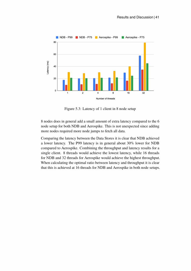
Results and Discussion | 41
Figure 5.3: Latency of 1 client in 8 node setup
8 nodes does in general add a small amount of extra latency compared to the 6node setup for both NDB and Aerospike. This is not unexpected since addingmore nodes required more node jumps to fetch all data.
Comparing the latency between the Data Stores it is clear that NDB achieveda lower latency. The P99 latency is in general about 30% lower for NDBcompared to Aerospike. Combining the throughput and latency results for asingle client. 8 threads would achieve the lowest latency, while 16 threadsfor NDB and 32 threads for Aerospike would achieve the highest throughput.When calculating the optimal ratio between latency and throughput it is clearthat this is achieved at 16 threads for NDB and Aerospike in both node setups.

42 |Results and Discussion
Figure 5.4: Client’s peak CPU in percentage for the 8 node setups
Observing Fig.5.4 it is clear that Aerospike experienced performance issueswith 32 threads because the client’s CPU utilization peaked at 100%. With16 threads the CPU was only utilized at around 70% which gave the clientsenough room to handle the Read requests directly as they were coming backfrom the Data Stores. For NDB the client’s CPU utilization stayed the samefor 16 and 32 threads. Thus the CPU was not the bottleneck for NDB whenraising the number of threads beyond 16. This indicates that one more clusterconnection could be used on the client side to raise the throughput, but this wasnever tested. The clients for NDB and Aerospike otherwise had very similarCPU utilization between 1 to 16 threads. But the NDB client being slightlymore effective because of the higher throughput observed in Fig.5.1. It shouldalso be noted that the overall CPU utilization of the clients was not affected bythe node setup.
An overall note about comparing the result between NDB and Aerospike is thatAerospike’s client API does the deserialization of the feature data. This is notdone with NDB’s API and thus something that needs to be done as a separatestep. This will add some extra computation to the NDB clients which cannotbe seen in this study. This computation overhead will however probably bequite small and constant.

Results and Discussion | 43
5.1.2 Several Clients
Based on the optimal number of threads found in Section 5.1.1 all clients used16 threads in this Read benchmark. The average throughput of the clients canbe observed in Fig.5.5.
When the number of clients increased average throughput for the Aerospikeclient rose steadily. There did however be a slight decrease with 8 clients and8 nodes. NDB’s average throughput was stable up to 4 clients in the 8 nodesetup, while there was a slight decrease between 2 and 4 clients in the 6 nodesetup. Going from 4 to 8 clients NDB suffered a throughput loss in the 8 nodesetup, while the 6 node setup maintain around the same throughput. ComparingNDB’s and Aerospike’s throughput, the same performance difference as couldbe seen with 1 client could be observed with 2 clients. The performancedifference was however a bit less with 4 clients in the 6 node setup and with 8clients in the 8 node setup, with 20% instead instead of the 35% observed with1 client.
Figure 5.5: Average throughput of the clients in both 6 and 8 node setup ofNDB and Aerospike
Looking at the Read benchmark tables for several clients in Appendix A itis interesting to note that there does seem to be some throughput unbalancebetween the clients. This problem appeared to be more severe for NDB’sclients where some clients got 20% less throughput. This problem was however

44 |Results and Discussion
less evident when using the 8 node setup. Aerospike also experienced theseperformance differences between the clients, but the differences was only atmost around 10%.
Figure 5.6: Average latency of the clients in 6 node setup for NDB andAerospike
Figure 5.7: Average latency of the clients in 8 node setup for NDB andAerospike

Results and Discussion | 45
Fig.5.6 shows how the batch Read latency were affected when adding moreclients in the 6 node setup. Aerospike’s latency was quite stable while NDB’sP99 latency increased for more than 2 clients in this node setup.
Fig.5.7 instead shows the latency performance with the 8 node setup. In thissetup the latency performance was more stable for NDB only increasing slightlyfor 8 clients. Aerospike did however suffer a slight latency increase already at2 and 4 clients, while 8 clients increased the P99 latency with 20% comparedto 4 clients. Comparing the P99 latency in the 8 node setup, NDB achieved ingeneral 35% lower latency.
Figure 5.8: CPU peak utilization in the Data Store in percentages
Observing Fig.5.8 it is clear that the Aerospike nodes were less utilized thanNDB’s data nodes for all client setups and that they seemed to scale better withthe clients. However, the throughput and latency results need to be taken intoconsideration when looking at this figure. Because NDB achieved around 20%higher throughput it is not unexpected that its data nodes are higher utilizedthan the Aerospike nodes. There is also a clear difference between the 6 and8 node setup for NDB, where 8 nodes are less utilized. The gap between thetwo node setups does appear to grow as the number of clients was increased.The same CPU utilization difference could not be observed with the Aerospikenodes as the 6 and 8 node setup had very similar peak CPU utilization.
NDB’s higher CPU utilization may also be partially explained by the fact that
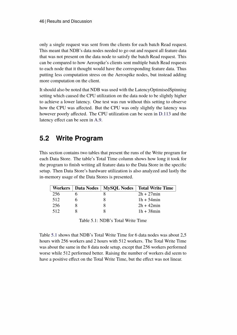
46 |Results and Discussion
only a single request was sent from the clients for each batch Read request.This meant that NDB’s data nodes needed to go out and request all feature datathat was not present on the data node to satisfy the batch Read request. Thiscan be compared to how Aerospike’s clients sent multiple batch Read requeststo each node that it thought would have the corresponding feature data. Thusputting less computation stress on the Aerospike nodes, but instead addingmore computation on the client.
It should also be noted that NDB was used with the LatencyOptimisedSpinningsetting which caused the CPU utilization on the data node to be slightly higherto achieve a lower latency. One test was run without this setting to observehow the CPU was affected. But the CPU was only slightly the latency washowever poorly affected. The CPU utilization can be seen in D.113 and thelatency effect can be seen in A.9.
5.2 Write Program
This section contains two tables that present the runs of the Write program foreach Data Store. The table’s Total Time column shows how long it took forthe program to finish writing all feature data to the Data Store in the specificsetup. Then Data Store’s hardware utilization is also analyzed and lastly thein-memory usage of the Data Stores is presented.
Workers Data Nodes MySQL Nodes Total Write Time256 6 8 2h + 27min512 6 8 1h + 54min256 8 8 2h + 42min512 8 8 1h + 38min
Table 5.1: NDB’s Total Write Time
Table 5.1 shows that NDB’s Total Write Time for 6 data nodes was about 2,5hours with 256 workers and 2 hours with 512 workers. The Total Write Timewas about the same in the 8 data node setup, except that 256 workers performedworse while 512 performed better. Raising the number of workers did seem tohave a positive effect on the Total Write Time, but the effect was not linear.

Results and Discussion | 47
Workers Data Nodes Total Write Time128 6 1h + 48min256 6 1h512 6 1 + 3min256 8 55min512 8 50min
Table 5.2: Aerospike’s Total Write Time
Investigating Aerospike’s write performance at Table 5.2 it is clear that its Writeperformance was a lot more efficient than NDB’s performance. The Total WriteTime seemed similar in both node setups. Shifting the number of workers inthe Dataflow only had an effect between 128 and 256 workers, where the effectalmost seemed to be linear for Total Write Time. The change between 256 and512 workers seemed negligible, even adding time in the case of the 6 nodesetup. For both 256 and 512 workers the write time was about 1 hour in bothnode setups.
Comparing the results between the Data Stores, Aerospike almost had the sameWrite time for 128 workers as NDB had for 512 workers. In the 8 node setupAerospike was about 70% faster than NDB for 256 workers and 45% for 512workers.
Figure 5.9: Data Store Cluster Nodes peak CPU in percentages

48 |Results and Discussion
Examining the Data Stores CPU utilization, see Fig.5.9, it is clear that NDBwasfar from hitting a bottleneck in terms of computation power during the Writeoperations. The 8 MySQL nodes used for inserting data into NDB seemedto take the higher CPU load. This was expected since these nodes needed toparse the SQL and send the data to the data nodes. Doubling the number ofWorkers did seem to almost double NDB’s data node CPU peak utilization,while only increasing the MySQL nodes peak CPU with 33%. This, togetherwith the Total Write Time effect observed in Table 5.1 suggests that the TotalWrite Time could decrease more by increasing the number of Workers passedthe point of 512.
Looking at Aerospike’s peak CPU utilization it was higher than that of NDB.This was not unexpected since the Aerospike nodes are handling a lot of theWrite computations per second. Taking into consideration how much less timeAerospike needed to Write all feature data it is clear that it is able to utilize itshardware resources more efficiently than NDB with this implementation. It isalso interesting to note that although increasing the number of Workers from256 to 512 gave a slight effect on the Total Write Time with about 5 minutes,the peak CPU of the Aerospike nodes increased with about 20%.
It should be noted that the overall Write implementation was probably notimplemented in the most efficient way for both NDB and Aerospike. Thisstudy focused on the properties that were most important for an OnlineFeature Store, which was how they handled Read workloads. Thus moreexperimentation on the Write implementation would probably yield moreefficient Write implementations.
NDB’s write performance was heavily affected by the number of MySQL nodesin the cluster setup. Giving more computation resources to the MySQL nodes,either horizontally or vertically, would probably also give a positive effect onNDB’s Total Write Time. One would also expect more efficient performanceif making use of batch inserts in SQL. Another thing that would most likelyincrease Write performance would be to use ClusterJ in the Write programinstead of using JDBC. This would also make the overall NDB cluster setup abit smaller, since it would only need one MySQL node to manage the settingsfor the tables. The main problem why this was not implemented in this studywas because ClusterJ requires the NDB C++ client on the same machine asClusterJ is executed. Making use of Dataflow jobs, generic machines weretemporarily spun up and loaded in with the Scala code. If one were to figureout a way to upload the NDB C++ client to these machines it would not behard to use ClusterJ instead of JDBC.
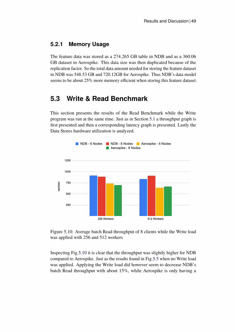
Results and Discussion | 49
5.2.1 Memory Usage
The feature data was stored as a 274.265 GB table in NDB and as a 360.06GB dataset in Aerospike. This data size was then duplicated because of thereplication factor. So the total data amount needed for storing the feature datasetin NDB was 548.53 GB and 720.12GB for Aerospike. Thus NDB’s data modelseems to be about 25% more memory efficient when storing this feature dataset.
5.3 Write & Read Benchmark
This section presents the results of the Read Benchmark while the Writeprogram was run at the same time. Just as in Section 5.1 a throughput graph isfirst presented and then a corresponding latency graph is presented. Lastly theData Stores hardware utilization is analyzed.
Figure 5.10: Average batch Read throughput of 8 clients while the Write loadwas applied with 256 and 512 workers
Inspecting Fig.5.10 it is clear that the throughput was slightly higher for NDBcompared to Aerospike. Just as the results found in Fig.5.5 when no Write loadwas applied. Applying the Write load did however seem to decrease NDB’sbatch Read throughput with about 15%, while Aerospike is only having a

50 |Results and Discussion
slight decrease in throughput. NDB’s throughput was however still higher thanAerospike’s when running the Write program with both 256 and 512 workers.A slight decrease in throughput could be seen when running with 512 workers,except with NDB in the 8 node setup that actually achieved a slightly betterthroughput result compared to 256 workers.
Figure 5.11: Average batch Read latency of the clients in both node setupswhile Write load was applied
Comparing Fig.5.11 with the results achieved when only doing batch Reads,see Fig.5.6 and Fig.5.7, it is clear that the latency was negatively affected whenwriting feature data at the same time as Reading. In NDB’s case the batch Readlatency was about 30% higher for both node setups.
The numbers shifted more between the Aerospike setups. There was only a10% difference between the 8 node setup. But for the 6 node setup the batchRead latency increased by 17% for 256 workers and 40% for 512 workers,compared to the numbers when only applying the Read workload.
NDB’s 8 node setup were able to handle more Write workers while maintaininga lower batch Read latency. It is also interesting to note that the P99 latency wasslightly higher for NDB with 256 workers in the 6 node setup, while the P75latency was higher for Aerospike. Apart from that run, NDB still achieved anoverall lower P99 and P75 latency than Aerospike. The performance differencewas however smaller than those observed when not applying the Write program

Results and Discussion | 51
at the same time. The difference now being around 15% compared to the 30-35% observed in Section 5.1.2. Raising the number of write workers did seemto have a negative effect on the Read performance with 8 clients for Aerospike.Which is interesting since as was observed previously, the Total Write Time forthe job did not change when raising the number of workers from 256 to 512workers.
Figure 5.12: The Data Stores Node’s peak CPU in percentages
Examining Fig.5.12 it is clear that Aerospike had a higher CPU peak, whichwas to be expected since its higher Write throughput. It is however interestingto compare these results with the peak CPU utilization observed when onlyapplying the Read or Write workload, see Fig.5.8 and Fig.5.9. The MySQLnode’s peak CPU utilization seems to be around the same levels as when onlyWriting data, which is to be expected since they are not affected by Readoperations. NDB’s data nodes have however almost double the peak CPU with256 workers in the 6 node setup. There was an expected utilization differencebetween the 6 and 8 node setup, where the later had a lower CPU peak, this gapwas however smaller with 512 workers. It is interesting to note that although256 workers had almost double the CPU peak, 512 workers was around thesame levels as was observed in Fig.5.9 when only Writing data.
Looking at Aerospike’s peak CPU utilization there was a clear differencebetween the node setups for 256 workers, but this disappears with 512 workers.It is also worth noting that Aerospike’s peak CPU was around 70% the same

52 |Results and Discussion
256 workers in the 6 node setup and for both node setups with 512 workers.This was around 10 percentage points lower than the peak CPU obtained whenjust Writing data.

Conclusions and Future Work | 53
Chapter 6
Conclusions and Future Work
In this chapter the thesis is concluded. The problem that has been addressed issummarized and a discussion is conducted regarding if the thesis managed toanswer the research question presented in the introduction. A short discussionis conducted regarding sustainability and ethics and lastly possible future workis discussed.
6.1 Conclusions
Several Data Stores were first investigated on how they would fit as the OnlineFeature Store component in Spotify’s system. A survey was conducted to findwhat Data Stores had been used before to implement Online Feature Stores.These Data Stores were then further examined based on their basic properties,scalability and performance. Several Data Stores were identified to satisfy thebasic requirements for being used as an Online Feature Store inside Spotify’sSearch system. However, looking at scalability and performance NDB andAerospike showed the best results based on previous benchmarks. These twoData Stores also had very different Data Models, NDB being RDBMS andAerospike being NoSQL Key-Value. This gave them both different propertiesthat were both good and bad for the Online Feature Store use-case. Thus NDBand Aerospike were chosen to be evaluated with Spotify Search’s Feature Dataas the Online Feature Store component. Because each request to the OnlineFeature Store required fetching the data for several features batch Read wasfound to provide big performance benefits. Thus the Online Feature Storeimplementations used batch Reads for both Data Stores.

54 |Conclusions and Future Work
Looking at the implemented Online Feature Stores Read performance NDBappeared to perform significantly better than Aerospike in terms of throughputand latency. It is even possible that further performance could have beenobtained from the NDB clients if one more API connection had been usedin NDB’s Java API. Looking at their scalability aspect none of the Readexperiments maxed out the Data Store node setups, it was always the number ofclients that was the bottleneck. Scaling the number of Read clients did howevercause a slight decrease in performance of NDB. Thus one can conclude thatthe NDB clients does not scale linearly up to 8 clients while the number ofAerospike clients does. One should however keep in mind that the NDB clientsstill had a higher throughput and a lower latency than the Aerospike clients.
Looking at the implementedOnline Feature StoresWrite performanceAerospikeclearly had the higher throughput. Because of limitations in the way NDB’sJava API could be used with Google Dataflow optimal Write performancecould never be tested for NDB. Instead MySQL nodes needed to be used whichadded an extra layer to NDB’s Write implementation, not being able to go tothe data layer directly. NDB did however still gave strong data consistency,while Aerospike only gave eventual data consistency. This became relevant inthe last experiment where the Read Workload was applied at the same timeas the Write workload. Having strong consistency one could be sure that allNDB clients read the same feature data, while this was only eventually true forAerospike. However, being that this is an Online Feature Store for Spotify’sSearch system, strong consistency is not a must since serving outdated featuredata will not be catastrophic in this use-case. It is clear that Read performancedeclines when the Write workload is applied for both Data Stores.
Thus we can conclude that both NDB and Aerospike can be implementedas an Online Feature Store component with Spotify Search’s feature data.NDB got the highest Read performance, which is the most important aspectof an Online Feature Store. It should however be taken into considerationthat significantly more work needed to be put into the NDB implementationcompared to Aerospike’s Online Feature Store implementation. Bottlenecksfound in the NDB’s Java client were addressed together with Logical Clocks,while no such work was conducted together with Aerospike.
It should be noted that the actual throughput and latency number should notbe taken as the maximum performance for these implementations. Becauseof the way the Data Store clusters were set up they were spread over threedifferent availability zones. This most likely caused decreases in performancefor both Data Stores when batch fetching required jumping between different

Conclusions and Future Work | 55
availability zones. Thus setting these clusters up with two availability zoneswould probably yield better performance for both Data Stores. The results arehowever comparable between the Data Stores since they both were benchmarkedin the same setup.
6.2 Sustainability and Ethics
Running Online Feature Stores is a relative cheap process compared todeveloping and training machine learning models. Dividing up the FeatureStore into an Online and Offline component does however provide sustainabilitybenefits. The Online Feature Store can run on high-end hardware while theOffline Feature Store works fine by running on cheaper hardware. This achievesboth economic and environmental sustainability.
Serving the wrong feature data can lead to big consequences depending whatthe machine learning model is predicting. In the case of this thesis the badimpact is very limited by possibly ranking an Artist too low or high in theSearch results. But say that the features instead were about predicting thepresence of cancer, then serving the wrong features could be catastrophic.
6.3 Future work
There are many more aspects of an Online Feature Store that could beinvestigated and there are also more Data Stores that could be evaluated againstthis use-case. In this section possible future work related to this thesis isproposed.
• Evaluate more Data Stores: With more time this thesis would have alsoevaluated Redis Cluster as an Online Feature Store. The reasoning forgoing with Redis Cluster was the big usage of Redis in Table 2.1 andits hinted ability to scale. Evaluating Redis Cluster would also make iteasier to compare the results of NDB and Aerospike against other DataStores, since Redis is such a widely used system.
• Find the limits of the Data Stores node setups: One would need to runthe Read experiments with more than 8 clients to find the limits of theData Stores in this setup. The Data Store’s CPU figures hint where this

56 |Conclusions and Future Work
limit could be, but both Data Stores did not appear to have a clear linearscaling in CPU usage.
• Investigate the clients further: What makes the NDB client able to getdouble the throughput compared to Aerospike with one thread? Whereis the extra time spent in the Aerospike client?
• Improve Write implementation: One can especially improve the Writeimplementation of NDB by using ClusterJ instead of JDBC. Likepreviously stated some work was put into trying to make ClusterJ workwith Google Dataflow, but this was never accomplished.
• More realistic cluster setups: To maximize the Data Stores performancethe clusters should have been set up in two different availability zoneswith replication. In this study the nodes were spread over three differentavailability zones. This caused a lot of extra added latency since thebatch fetching data may have required jumping over different zones.

REFERENCES | 57
References
[1] DC@KTH, Feature Store for ML, (accessed September 30, 2020), https://www.featurestore.org/.
[2] Logical Clocks, Hopsworks Feature Store, (accessed September 15,2020), https://uploads-ssl.webflow.com/5e6f7cd3ee7f51d539a4da0b/5ef397dce942172c90259858_feature%20management%20platform%20v02.pdf.
[3] FEAST, Architecture, (accessed September 15, 2020), https://docs.feast.dev/user-guide/architecture.
[4] W. Pienaar, “Feast: Feature store for machine learning,” 2019,anthill Inside 2019 https://hasgeek.com/anthillinside/2019/proposals/feast-feature-store-for-machine-learning-HBMmchibhze5ZpWqzhcian.
[5] J. Hermann, Michelangelo - Machine Learning @Uber, Mar 23, 2019,qCon https://www.infoq.com/presentations/uber-ml-michelangelo/?utm_source=youtube&utm_medium=link&utm_campaign=qcontalks.
[6] J. Hermann and M. D. Balso, Meet Michelangelo: Uber’s MachineLearning Platform, 2017 (accessed September 30, 2020), https://eng.uber.com/michelangelo-machine-learning-platform/.
[7] V. Zanoyan and E. Shapiro, “Zipline—airbnb’s declarativefeature engineering framework,” Okt 21, 2019, databrickshttps://www.youtube.com/watch?v=iUnO4MLAGDU&feature=emb_title&ab_channel=Databricks.
[8] N. Sarwar, “Operationalizing machine learning—managingprovenance from raw data to predictions,” 2018, databrickshttps://www.youtube.com/watch?v=iUnO4MLAGDU&feature=emb_title&ab_channel=Databricks.

58 |REFERENCES
[9] R. Romano, “Overview of wix’s machine learning platform,” Feb18, 2020, wix Engineering Tech Talks https://www.youtube.com/watch?v=E8839ENL-WY&feature=emb_title&ab_channel=WixEngineeringTechTalks.
[10] N. Jain, “Real time machine learning inference platform,” Nov 27,2020, hagsgeekhttps://hasgeek.com/rootconf/2020-delhi/proposals/real-time-machine-learning-inference-platform-zoma-Jpk3vdwjcrQKGs19mGLibj.
[11] S. Khadder, “Feature stores: Building machine learninginfrastructure on apache pulsar,” Jun 24, 2020, pulsar Summit2020 https://www.youtube.com/watch?v=eLJk5sOME0o&feature=emb_title&ab_channel=StreamNative.
[12] S. Canchi and T. Wenzel, Managing ML Models @ Scale - Intuit’sML Platform, Jul. 2020, https://www.usenix.org/conference/opml20/presentation/wenzel.
[13] S. Bathini, “Sony interactive entertainment: Powering playstationpersonalization to millions,” Jun 17, 2020, aerospike SUMMIT’20 https://www.aerospike.com/resources/videos/summit20/sony-powering-playstation-personalization-to-millions/.
[14] J. Han, E. Haihong, G. Le, and J. Du, “Survey on nosql database,” in 20116th international conference on pervasive computing and applications.IEEE, 2011, pp. 363–366.
[15] A. Makris, K. Tserpes, V. Andronikou, and D. Anagnostopoulos, “Aclassification of nosql data stores based on key design characteristics.” inCloud Forward, 2016, pp. 94–103.
[16] G. Belalem, H. Matallah, and K. Bouamrane, “Evaluation of nosqldatabases: Mongodb, cassandra, hbase, redis, couchbase, orientdb,”International journal of software science and computational intelligence,vol. 12, no. 4, pp. 71–91, 2020.
[17] N. Jatana, S. Puri, M. Ahuja, I. Kathuria, and D. Gosain, “A surveyand comparison of relational and non-relational database,” InternationalJournal of Engineering Research & Technology, vol. 1, no. 6, pp. 1–5,2012.
[18] F. Gessert and N. Ritter, “Scalable data management: Nosql data storesin research and practice,” in 2016 IEEE 32nd International Conferenceon Data Engineering (ICDE). IEEE, 2016, pp. 1420–1423.

REFERENCES | 59
[19] A. Fox, S. D. Gribble, Y. Chawathe, E. A. Brewer, and P. Gauthier,“Cluster-based scalable network services,” in Proceedings of the sixteenthACM symposium on Operating systems principles, 1997, pp. 78–91.
[20] M. Kleppmann, Designing Data-Intensive Applications: The Big IdeasBehind Reliable, Scalable, and Maintainable Systems. Sebastopol:O’Reilly Media, Incorporated, 2017. ISBN 1449373321
[21] T. Weiss, MySQL acquiring data management system vendorAlzato, Oct 2003, https://www.computerworld.com/article/2572959/mysql-acquiring-data-management-system-vendor-alzato.html.
[22] R. Cattell, “Scalable sql and nosql data stores,” Acm Sigmod Record,vol. 39, no. 4, pp. 12–27, 2011.
[23] Oracle, Chapter 4 MySQL NDB Cluster Connector for Java, (accessedFeb 5, 2021), https://dev.mysql.com/doc/ndbapi/en/mccj.html.
[24] B. Ocklin, “Sql faster than nosql, mysql ndb 8.0,” Jan31, 2020, oracle https://www2.slideshare.net/ocklin/mysql-ndb-cluster-80-sql-faster-than-nosql.
[25] Aerospike, Aerospike Technical Documentation, 2020 (accessed October2, 2020), https://www.aerospike.com/docs/#.
[26] Aerospike, Database Product Matrix, 2020 (accessed October 2, 2020),https://www.aerospike.com/products/product-matrix/.
[27] D. Gembalczyk, F. M. Schuhknecht, and J. Dittrich, “An experimentalanalysis of different key-value stores and relational databases,”Datenbanksysteme für Business, Technologie und Web (BTW 2017), 2017.
[28] K. Kingsbury, “Redis-raft 1b3fbf6,” Jun 23, 2020 (accessed October 1,2020), aphyr https://jepsen.io/analyses/redis-raft-1b3fbf6.
[29] ——, “Jepsen: Redis,” 2013 (accessed October 1, 2020), aphyr https://aphyr.com/posts/283-call-me-maybe-redis.
[30] Redis, Redis Cluster Specification, (accessed September 30, 2020), https://redis.io/topics/cluster-spec.
[31] Google Cloud, Overview of Memorystore for Redis, (accessedOctober 2, 2020), https://cloud.google.com/memorystore/docs/redis/redis-overview.

60 |REFERENCES
[32] G. DeCandia, D. Hastorun, M. Jampani, G. Kakulapati, A. Lakshman,A. Pilchin, S. Sivasubramanian, P. Vosshall, and W. Vogels, “Dynamo,”Operating systems review, vol. 41, no. 6, p. 205, 2007.
[33] riak, Riak KV 2.2.3, (accessed October 2, 2020), https://docs.riak.com/riak/kv/2.2.3/.
[34] F. Chang, J. Dean, S. Ghemawat, W. C. Hsieh, D. A.Wallach, M. Burrows,T. Chandra, A. Fikes, and R. E. Gruber, “Bigtable: A distributed storagesystem for structured data,” ACM Transactions on Computer Systems(TOCS), vol. 26, no. 2, pp. 1–26, 2008.
[35] Apache HBase,Welcome to Apache HBase™, (accessed October 5, 2020),http://hbase.apache.org/.
[36] Netflix, Introduction, (accessed September 19, 2020), https://hollow.how/.
[37] R. Srinivas, Q&A with Drew Koszewnik on a Disseminated Cache,Netflix Hollow, Dec 2016, https://www.infoq.com/news/2016/12/announcing-netflix-hollow/.
[38] B. F. Cooper, A. Silberstein, E. Tam, R. Ramakrishnan, and R. Sears,“Benchmarking cloud serving systems with ycsb,” in Proceedings of the1st ACM symposium on Cloud computing, 2010, pp. 143–154.
[39] B. Cooper, YCSB, (accessed September 30, 2020), https://github.com/brianfrankcooper/YCSB.
[40] K. Kingsbury, Jepsen, (accessed September 30, 2020), https://github.com/jepsen-io/jepsen.
[41] ——, Jepsen: Aerospike, 2015 (accessed October 1, 2020), aphyr https://aphyr.com/posts/324-jepsen-aerospike.
[42] ——, “Jepsen: Aerospike,” 2018 (accessed September 30, 2020), aphyrhttps://jepsen.io/analyses/aerospike-3-99-0-3.
[43] ——, “Jepsen 9: A fsyncing feeling,” May 8, 2018 (accessed October 1,2020), gOTO 2018 https://www.youtube.com/watch?v=tRc0O9VgzB0&ab_channel=GOTOConferences.
[44] The Apache Software Foundation, “Apache beam: An advanced unifiedprogramming model,” (accessed January 19, 2021), https://beam.apache.org/.

REFERENCES | 61
[45] Spotify, “Scio,” 2020 (accessed January 19, 2021), https://spotify.github.io/scio/.

62 | Benchmark Tables
Appendix A
Benchmark Tables
A.1 Read Benchmark
A.1.1 NDB
Number of threads Average Throughput (ops/sec) P99 Latency (ms) P75 Latency (ms) P50 Latency (ms)1 122 16.8 9.1 8.62 225 18.1 10 9.14 420 19.7 10.9 9.78 777 21.7 12.3 10.316 1189 28.1 15.6 13.632 1164 53 32.3 27.1
Table A.1: 1 client & 6 Data Nodes
Client Average Throughput (ops/sec) P99 Latency (ms) P75 Latency (ms) P50 Latency (ms)1 1175 29 15.8 13.72 1131 29.9 16.4 14.2Average: 1153 29.5 16.1 14
Table A.2: 2 clients, 16 threads & 6 data nodes

Benchmark Tables | 63
Client Average Throughput (ops/sec) P99 Latency (ms) P75 Latency (ms) P50 Latency (ms)1 1120 39.6 16.2 13.72 1020 43.7 17.8 153 851 48.5 21.8 17.94 1086 42.1 16.6 14Average: 1019 43.5 18.1 15.2
Table A.3: 4 clients, 16 threads & 6 data nodes
Client Average Throughput (ops/sec) P99 Latency (ms) P75 Latency (ms) P50 Latency (ms)1 1070 35.3 17.4 14.62 1012 36.7 18.4 15.43 850 41.9 22.2 18.54 850 33.8 17.2 14.55 885 39.8 21.2 17.66 1093 36 16.9 14.17 1058 37.6 17.5 14.68 1116 34.7 16.5 13.9Average: 992 37 18.4 15.4
Table A.4: 8 clients, 16 threads & 6 data nodes
Number of threads Average Throughput (ops/sec) P99 Latency (ms) P75 Latency (ms) P50 Latency (ms)1 116 17.7 9.6 8.92 210 20.4 10.7 9.74 407 20.6 11.3 9.98 772 21.7 12.1 10.416 1111 29.7 16.5 14.532 1086 57.9 34.8 29
Table A.5: 1 client & 8 Data Nodes
Client Average Throughput (ops/sec) P99 Latency (ms) P75 Latency (ms) P50 Latency (ms)1 1191 27.5 15.5 13.62 1183 27.7 15.7 13.7Average: 1187 27.6 15.6 13.7
Table A.6: 2 clients, 16 threads & 8 data nodes

64 | Benchmark Tables
Client Average Throughput (ops/sec) P99 Latency (ms) P75 Latency (ms) P50 Latency (ms)1 1209 27.1 15.3 13.42 1202 27.4 15.4 13.53 1074 31.7 17.3 14.94 1218 27.4 15.2 13.3Average: 1176 28.4 15.8 13.8
Table A.7: 4 clients, 16 threads & 8 data nodes
Client Average Throughput (ops/sec) P99 Latency (ms) P75 Latency (ms) P50 Latency (ms)1 1050 36.5 17.5 14.82 1043 36.5 17.6 14.93 981 38 19 164 1070 36 17.2 14.55 1044 36.5 17.6 14.96 1117 34.5 16.4 13.97 1081 36 17 14.48 1081 36 16.9 14.4Average: 1058 36.3 17.4 14.7
Table A.8: 8 clients, 16 threads & 8 data nodes
Client Average Throughput (ops/sec) P99 Latency (ms) P75 Latency (ms) P50 Latency (ms)1 906 45.7 20.8 16.52 776 52.3 24.3 19.33 803 49.9 23.6 18.94 842 46.7 22.5 17.95 897 46.4 21.1 16.66 951 44.4 19.9 15.67 866 48.4 22 16.88 941 45.2 20 15.7Average: 873 41.7 22 17.2
Table A.9: 8 clients, 16 threads & 6 data nodes without spinning

Benchmark Tables | 65
A.1.2 Aerospike
Number of threads Average Throughput (ops/sec) P99 Latency (ms) P75 Latency (ms) P50 Latency (ms)1 60 28.5 19.8 17.32 118 28.4 20.3 17.74 243 28.3 19.9 17.28 461 31.3 21 1816 785 39.2 24.7 2132 933 68 40.5 34.5
Table A.10: 1 client & 6 Aerospike Nodes
Client Average Throughput (ops/sec) P99 Latency (ms) P75 Latency (ms) P50 Latency (ms)1 793 42.3 24.3 20.62 773 41 25 21.3Average: 783 41.15 24.65 20.95
Table A.11: 2 clients, 16 threads & 6 data nodes
Client Average Throughput (ops/sec) P99 Latency (ms) P75 Latency (ms) P50 Latency (ms)1 942 70.1 40 33.82 910 71.3 41.5 35.2Average: 926 70.7 40.8 34.5
Table A.12: 2 clients, 32 threads & 6 data nodes
Client Average Throughput (ops/sec) P99 Latency (ms) P75 Latency (ms) P50 Latency (ms)1 815 40 23.8 20.12 821 39.8 23.5 19.93 761 42.5 25.5 21.54 801 39.6 24.2 20.5Average: 800 40.5 24.3 20.5
Table A.13: 4 clients, 16 threads & 6 data nodes

66 | Benchmark Tables
Client Average Throughput (ops/sec) P99 Latency (ms) P75 Latency (ms) P50 Latency (ms)1 825 38.2 23.5 19.92 803 39.7 24.2 20.43 779 41 24.8 214 808 39.5 24 20.25 799 40.2 24.2 20.46 858 35 23 19.37 862 35 22.9 19.18 796 40 24.6 21Average: 816 38.6 23.9 20.2
Table A.14: 8 clients, 16 threads & 6 data nodes
Number of threads Average Throughput (ops/sec) P99 Latency (ms) P75 Latency (ms) P50 Latency (ms)1 55 30.8 21.3 18.92 116 29 20.5 17.94 226 30.3 21.3 18.58 441 32.8 21.8 18.816 774 40.2 24.9 21.232 823 79.2 45.4 38.9
Table A.15: 1 client & 8 Aerospike Nodes
Client Average Throughput (ops/sec) P99 Latency (ms) P75 Latency (ms) P50 Latency (ms)1 743 44 25.8 222 739 44 25.9 22.1Average: 741 44 25.9 22.1
Table A.16: 2 clients, 16 threads & 8 data nodes
Client Average Throughput (ops/sec) P99 Latency (ms) P75 Latency (ms) P50 Latency (ms)1 761 40.8 25.3 21.62 753 44.6 25.4 21.63 678 47.9 28.1 244 772 40.1 24.9 21.3Average: 741 43.4 25.9 22.1
Table A.17: 4 clients, 16 threads & 8 data nodes

Benchmark Tables | 67
Client Average Throughput (ops/sec) P99 Latency (ms) P75 Latency (ms) P50 Latency (ms)1 685 53.1 27.4 232 641 56.5 29.1 24.53 648 55.5 28.9 24.24 648 55.5 28.9 24.25 687 53.1 27.2 22.96 707 52.9 26.3 22.17 690 52.9 27 22.78 697 52.8 26.8 22.5Average: 675 53.8 27.7 23.3
Table A.18: 8 clients, 16 threads & 8 data nodes
A.2 Read & Write Benchmark
A.2.1 NDB
Client Average Throughput (ops/sec) P99 Latency (ms) P75 Latency (ms) P50 Latency (ms)1 952 48.2 19.9 15.62 906 49 20.9 16.53 811 50.5 23.5 18.84 923 51.6 20.4 165 839 55.2 22.6 17.96 976 46.2 19.5 157 932 51.7 20.2 15.88 982 45.7 19.4 15Average: 915 49.8 20.8 16.3
Table A.19: 256 workers, 8 clients, 16 threads, 8 MySQL & 6 data nodes

68 | Benchmark Tables
Client Average Throughput (ops/sec) P99 Latency (ms) P75 Latency (ms) P50 Latency (ms)1 848 56.8 22.4 16.72 825 58.7 22.9 17.33 744 61.3 25.5 19.84 876 54.1 21.8 16.45 749 59.7 25.5 19.66 891 54.1 21.5 15.97 879 54.1 21.8 16.28 888 55.3 21.5 15.8Average: 838 56.8 22.9 17.2
Table A.20: 512 workers, 8 clients, 16 threads, 8 MySQL & 6 data nodes
Client Average Throughput (ops/sec) P99 Latency (ms) P75 Latency (ms) P50 Latency (ms)1 939 48.4 19,5 15.72 935 48.8 19.6 15.73 785 52.4 23.8 19.34 888 50 20.8 16.95 902 49.2 20.4 16.46 919 49 20 16.17 769 53.8 24.7 19.28 967 47.5 18.9 15.1Average: 888 49.4 21 16.8
Table A.21: 256 workers, 8 clients, 16 threads, 8 MySQL & 8 data nodes
Client Average Throughput (ops/sec) P99 Latency (ms) P75 Latency (ms) P50 Latency (ms)1 960 48.2 19.1 15.52 934 52 19.6 15.83 835 51.2 22.3 18.34 876 51.9 21.1 17.25 922 50.3 20 16.36 943 51.1 19.4 15.87 831 52.5 22.5 18.38 986 48 18.7 15.1Average: 911 50.7 20 16.5
Table A.22: 512 workers, 8 clients, 16 threads, 8 MySQL & 8 data nodes

Benchmark Tables | 69
A.2.2 Aerospike
Client Average Throughput (ops/sec) P99 Latency (ms) P75 Latency (ms) P50 Latency (ms)1 751 46.1 25.3 21.62 752 43.1 25.5 21.73 651 52.3 29.2 24.84 752 42.3 25.4 21.75 739 43 26 226 764 43.5 25.3 21.47 779 39.6 24.8 21.18 698 54.6 27.3 23.2Average: 736 45.6 29.5 22.2
Table A.23: 256 workers, 8 clients, 16 threads & 6 data nodes
Client Average Throughput (ops/sec) P99 Latency (ms) P75 Latency (ms) P50 Latency (ms)1 663 60.5 27.9 23.42 647 62.7 28.5 243 606 65 30.5 25.64 646 62.3 28.6 245 649 63 28.5 23.86 653 61.1 28.3 23.87 594 67.3 31.5 25.98 669 60.3 27.7 23.9Average: 641 62.8 28.9 24.3
Table A.24: 512 workers, 8 clients, 16 threads & 6 data nodes
Client Average Throughput (ops/sec) P99 Latency (ms) P75 Latency (ms) P50 Latency (ms)1 718 54.8 26.1 22.22 697 58.1 26.9 22.93 635 59.5 29.6 25.14 712 55.3 26.3 22.35 664 58 28.3 246 728 54.4 25.8 21.87 704 56.2 26.6 22.68 732 53.3 25.7 21.8Average: 699 56.2 26.9 22.8
Table A.25: 256 workers, 8 clients, 16 threads & 8 data nodes

70 | Benchmark Tables
Client Average Throughput (ops/sec) P99 Latency (ms) P75 Latency (ms) P50 Latency (ms)1 682 56.6 27.4 23.12 655 65.7 28.1 23.73 612 61.4 30.5 25.84 680 57.7 27.4 23.15 660 58 28.3 23.96 698 55.8 26.7 22.57 674 62 27.4 23.28 692 54.1 27.1 21Average: 669 58.9 27.9 23.3
Table A.26: 512 workers, 8 clients, 16 threads & 8 data nodes

Cluster Configurations | 71
Appendix B
Cluster Configurations
B.1 NDB Configuration
[ ndbd d e f a u l t ]NoOfRepl icas =2DataMemory=185G
LockPagesInMainMemory=1
TcpBind_INADDR_ANY=FALSENoOfFragmentLogPar ts =16NoOfFragmentLogFi les =16F r agmen tLogF i l eS i z e =16MMaxNoOfTables =4096MaxNoOfOrderedIndexes =2048MaxNoOfUniqueHashIndexes =512MaxNoOfTriggers =2048MaxDMLOpera t ionsPerTransac t ion =4294967295Transac t i onBuf f e rMemory =1MMaxPa r a l l e l S c an sPe rF r agmen t =256MaxDiskWriteSpeed=20MMaxDiskWr i t eSpeedOthe rNodeRes ta r t =50MMaxDiskWri teSpeedOwnRestar t =200MMinDiskWri teSpeed =10MRedoBuf fe r =32M

72 |Cluster Configurations
LongMessageBuffer =64MMaxFKBuildBatchSize =64T r a n s a c t i o n I n a c t i v e T im e o u t =1500T r a n s a c t i o nDead l o c kDe t e c t i o nT imeou t =1500Rea lT imeSchedu l e r =0CompressedLCP=0CompressedBackup=1MaxAl loca te =32MDefau l tHashMapSize =3840ODi rec t =0ExtraSendBufferMemory=0Tota lSendBufferMemory =16MD i s kP a g eBu f f e r E n t r i e s =10DiskPageBufferMemory =512MSharedGlobalMemory =2048MDiskIOThreadPool =32DiskSyncS ize =4M
MaxNoOfConcurrentScans =500MaxNoOfConcur ren tOpera t ions =200000MaxNoOfConcur r en tTransac t ions =16192MaxNoOfAt t r ibu tes =5000
MaxReorgBui ldBatchSize =64En a b l e P a r t i a l L c p =1RecoveryWork=60Inse r tRecove ryWork =40
#Opt imize f o r t h r o u ghpu t : 0 ( r ange 0 . . 1 0 )SpinMethod=La t en cyOp t im i s edSp i nn i ngS ch edu l e rRe s pon s i v e n e s s =5Schedu l e rExe cu t i o nT ime r =50
Bu i l d I nd exTh r e ad s =128TwoPa s s I n i t i a lNodeRe s t a r tCopy= t r u eNuma=1
MaxNoOfExecut ionThreads =32

Cluster Configurations | 73
S t a r t F a i l u r e T im e o u t =0
Star tNoNodeGroupTimeout =0
S t a r t P a r t i a l T i m e o u t =0
S t a r t P a r t i t i o n e d T im e o u t =0
[ ndb_mgmd ]# Management p r o c e s s o p t i o n s :HostName= # Hostname of management nodeDa taDi r = / va r / l i b / mysql − c l u s t e r
[ ndbd ]# Op t i on s f o r d a t a node "B" :HostName=NodeId=2 # Node ID f o r t h i s d a t a nodeDa taDi r = / u s r / l o c a l / mysql / d a t a
[ ndbd ]# Op t i on s f o r d a t a node "B" :HostName=NodeId=3 # Node ID f o r t h i s d a t a nodeDa taDi r = / u s r / l o c a l / mysql / d a t a
[ ndbd ]# Op t i on s f o r d a t a node "B" :HostName=NodeId=4 # Node ID f o r t h i s d a t a nodeDa taDi r = / u s r / l o c a l / mysql / d a t a
[ ndbd ]# Op t i on s f o r d a t a node "B" :HostName=NodeId=5 # Node ID f o r t h i s d a t a nodeDa taDi r = / u s r / l o c a l / mysql / d a t a
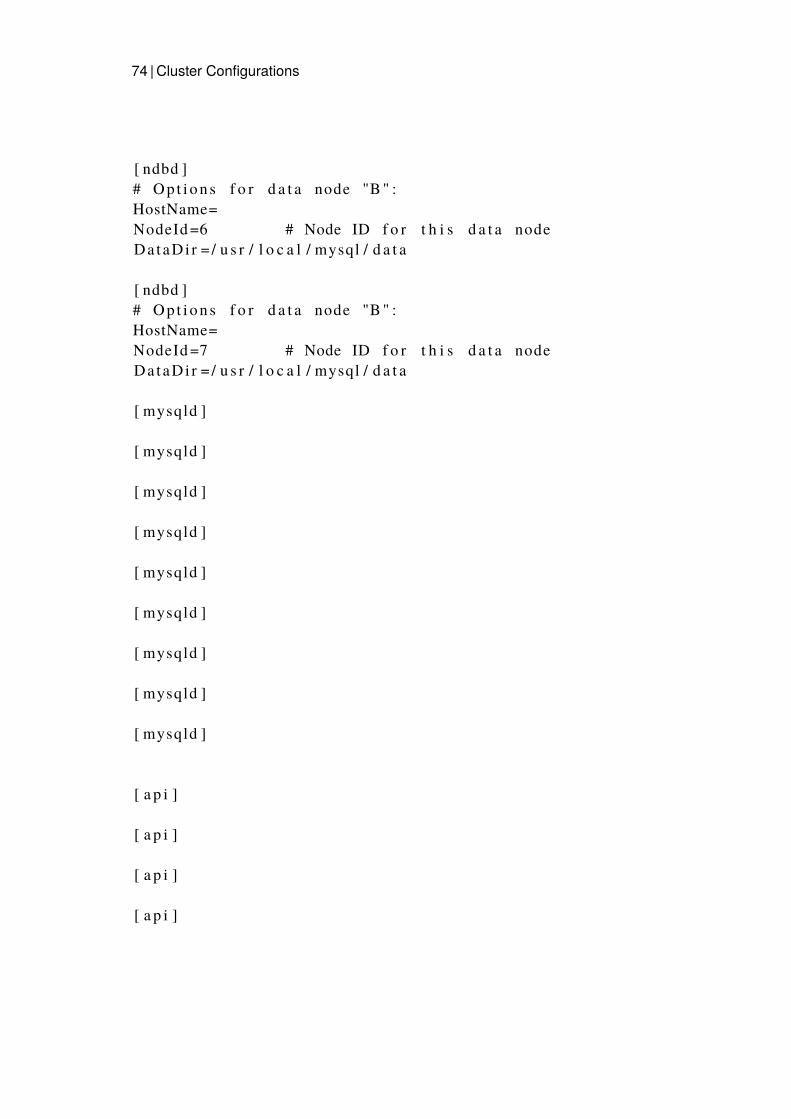
74 |Cluster Configurations
[ ndbd ]# Op t i on s f o r d a t a node "B" :HostName=NodeId=6 # Node ID f o r t h i s d a t a nodeDa taDi r = / u s r / l o c a l / mysql / d a t a
[ ndbd ]# Op t i on s f o r d a t a node "B" :HostName=NodeId=7 # Node ID f o r t h i s d a t a nodeDa taDi r = / u s r / l o c a l / mysql / d a t a
[ mysqld ]
[ mysqld ]
[ mysqld ]
[ mysqld ]
[ mysqld ]
[ mysqld ]
[ mysqld ]
[ mysqld ]
[ mysqld ]
[ a p i ]
[ a p i ]
[ a p i ]
[ a p i ]
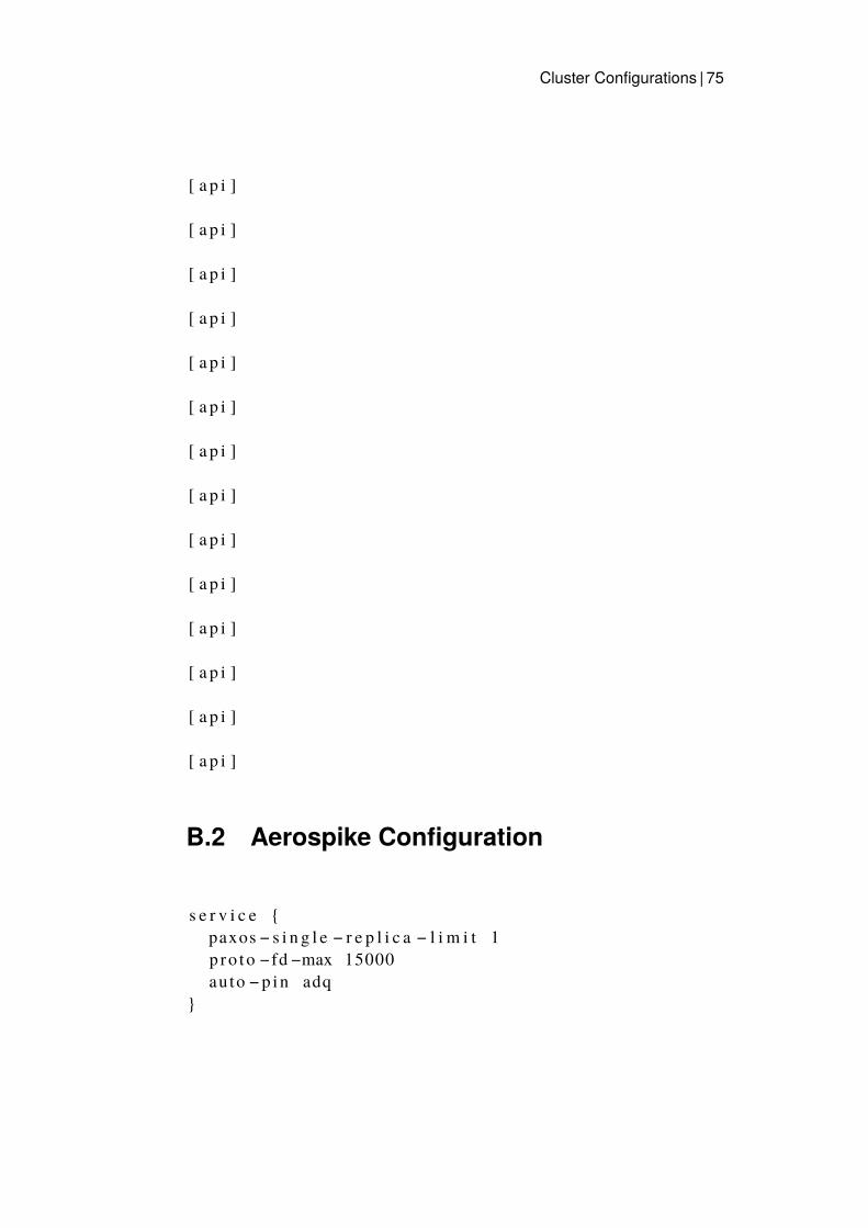
Cluster Configurations | 75
[ a p i ]
[ a p i ]
[ a p i ]
[ a p i ]
[ a p i ]
[ a p i ]
[ a p i ]
[ a p i ]
[ a p i ]
[ a p i ]
[ a p i ]
[ a p i ]
[ a p i ]
[ a p i ]
B.2 Aerospike Configuration
s e r v i c e {paxos − s i n g l e − r e p l i c a − l i m i t 1p ro to − fd −max 15000auto −p in adq
}

76 |Cluster Configurations
l o g g i n g {con s o l e {
c o n t e x t any i n f o}
}
ne twork {s e r v i c e {
a d d r e s s anyp o r t 3000
}
h e a r t b e a t {mode mesha d d r e s s REPLACE_MEpo r t 3002 # He a r t b e a t p o r t f o r t h i s node .
i n t e r v a l 250t imeou t 20
}
f a b r i c {p o r t 3001
}
i n f o {p o r t 3003
}}
namespace expe r imen t {r e p l i c a t i o n − f a c t o r 2memory− s i z e 204G
s t o r a g e − eng i n e d ev i c e {f i l e / op t / a e r o s p i k e / d a t a / t e s t . d a t a
f i l e s i z e 800G

Cluster Configurations | 77
da ta − in −memory t r u e}
}

78 | Availability Zones
Appendix C
Availability Zones
C.1 NDB
Data Node Availability Zone1 d2 d3 b4 b5 c6 c
Table C.1: Availability zones of 6 NDB data node setup
Data Node Availability Zone1 b2 b3 b4 c5 c6 c7 d8 d
Table C.2: Availability zones of 8 NDB data node setup

Availability Zones | 79
MySQL Node Availability Zone1 b2 b3 c4 c5 c6 d7 d8 d
Table C.3: Availability zones of 8 MySQL node setup
C.2 Aerospike
Data Node Availability Zone1 b2 b3 c4 c5 d6 d
Table C.4: Availability zones of 6 Aerospike node setup
Data Node Availability Zone1 b2 b3 c4 c5 c6 d7 d8 d
Table C.5: Availability zones of 8 Aerospike node setup

80 |Hardware Utilization
Appendix D
Hardware Utilization
D.1 Read Benchmark
D.1.1 1 Client, 6 Nodes & 1 Thread
NDB
Figure D.1: Client Max CPU

Hardware Utilization | 81
Figure D.2: Client Bandwidth Sent
Figure D.3: Client Bandwidth Received
Figure D.4: NDB Max CPU

82 |Hardware Utilization
Figure D.5: NDB Bandwidth Sent
Figure D.6: NDB Bandwidth Received
Aerospike
Figure D.7: Client Max CPU

Hardware Utilization | 83
Figure D.8: Client Bandwidth Sent
Figure D.9: Client Bandwidth Received
Figure D.10: Aerospike Max CPU
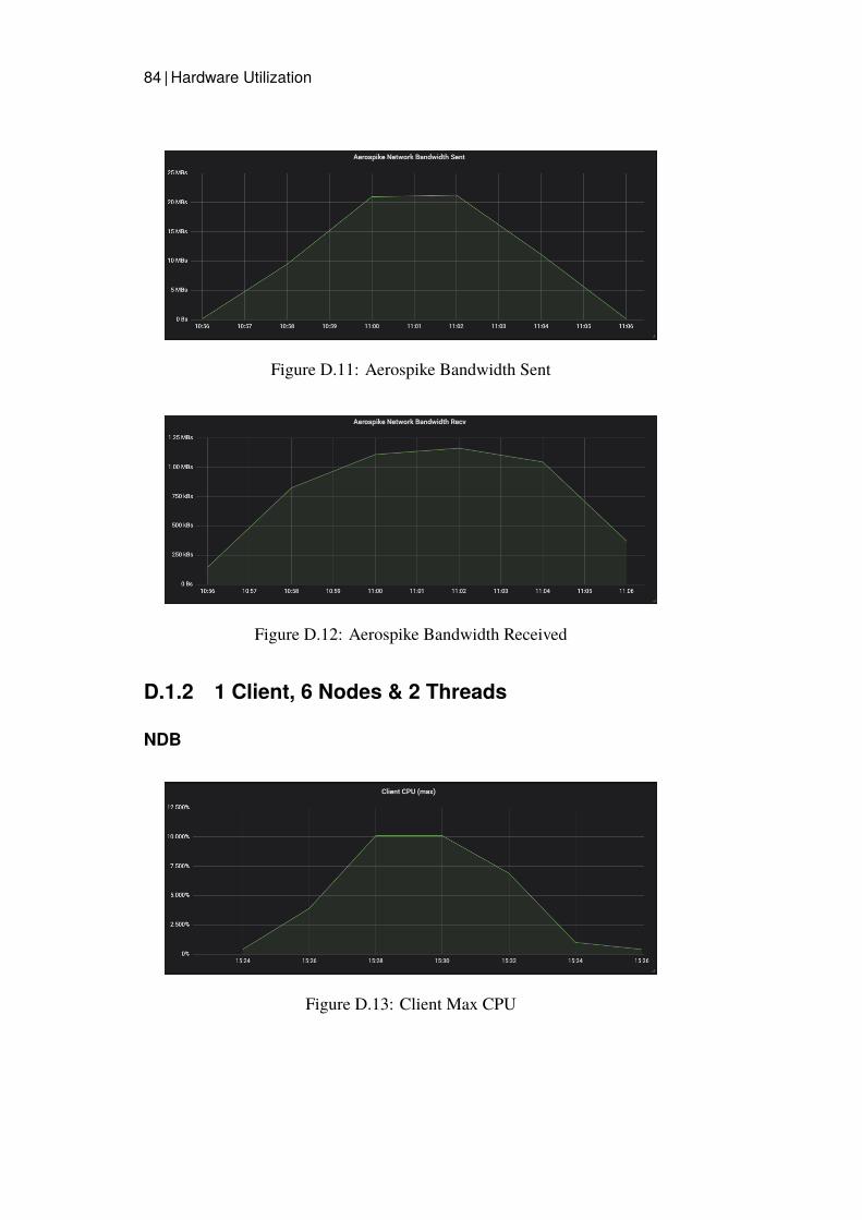
84 |Hardware Utilization
Figure D.11: Aerospike Bandwidth Sent
Figure D.12: Aerospike Bandwidth Received
D.1.2 1 Client, 6 Nodes & 2 Threads
NDB
Figure D.13: Client Max CPU

Hardware Utilization | 85
Figure D.14: Client Bandwidth Sent
Figure D.15: Client Bandwidth Received
Figure D.16: NDB Max CPU

86 |Hardware Utilization
Figure D.17: NDB Bandwidth Sent
Figure D.18: NDB Bandwidth Received
Aerospike
Figure D.19: Client Max CPU

Hardware Utilization | 87
Figure D.20: Client Bandwidth Sent
Figure D.21: Client Bandwidth Received
Figure D.22: Aerospike Max CPU

88 |Hardware Utilization
Figure D.23: Aerospike Bandwidth Sent
Figure D.24: Aerospike Bandwidth Received
D.1.3 1 Client, 6 Nodes & 4 Threads
NDB
Figure D.25: Client Max CPU

Hardware Utilization | 89
Figure D.26: Client Bandwidth Sent
Figure D.27: Client Bandwidth Received
Figure D.28: NDB Max CPU

90 |Hardware Utilization
Figure D.29: NDB Bandwidth Sent
Figure D.30: NDB Bandwidth Received
Aerospike
Figure D.31: Client Max CPU

Hardware Utilization | 91
Figure D.32: Client Bandwidth Sent
Figure D.33: Client Bandwidth Received
Figure D.34: Aerospike Max CPU

92 |Hardware Utilization
Figure D.35: Aerospike Bandwidth Sent
Figure D.36: Aerospike Bandwidth Received
D.1.4 1 Client, 6 Nodes & 8 Threads
NDB
Figure D.37: Client Max CPU

Hardware Utilization | 93
Figure D.38: Client Bandwidth Sent
Figure D.39: Client Bandwidth Received
Figure D.40: NDB Max CPU

94 |Hardware Utilization
Figure D.41: NDB Bandwidth Sent
Figure D.42: NDB Bandwidth Received
Aerospike
Figure D.43: Client Max CPU

Hardware Utilization | 95
Figure D.44: Client Bandwidth Sent
Figure D.45: Client Bandwidth Received
Figure D.46: Aerospike Max CPU

96 |Hardware Utilization
Figure D.47: Aerospike Bandwidth Sent
Figure D.48: Aerospike Bandwidth Received
D.1.5 1 Client, 6 Nodes & 16 Threads
NDB
Figure D.49: Client Max CPU

Hardware Utilization | 97
Figure D.50: Client Bandwidth Sent
Figure D.51: Client Bandwidth Received
Figure D.52: NDB Max CPU

98 |Hardware Utilization
Figure D.53: NDB Bandwidth Sent
Figure D.54: NDB Bandwidth Received
Aerospike
Figure D.55: Client Max CPU

Hardware Utilization | 99
Figure D.56: Client Bandwidth Sent
Figure D.57: Client Bandwidth Received
Figure D.58: Aerospike Max CPU

100 |Hardware Utilization
Figure D.59: Aerospike Bandwidth Sent
Figure D.60: Aerospike Bandwidth Received
D.1.6 1 Client, 6 Nodes & 32 Threads
NDB
Figure D.61: Client Max CPU
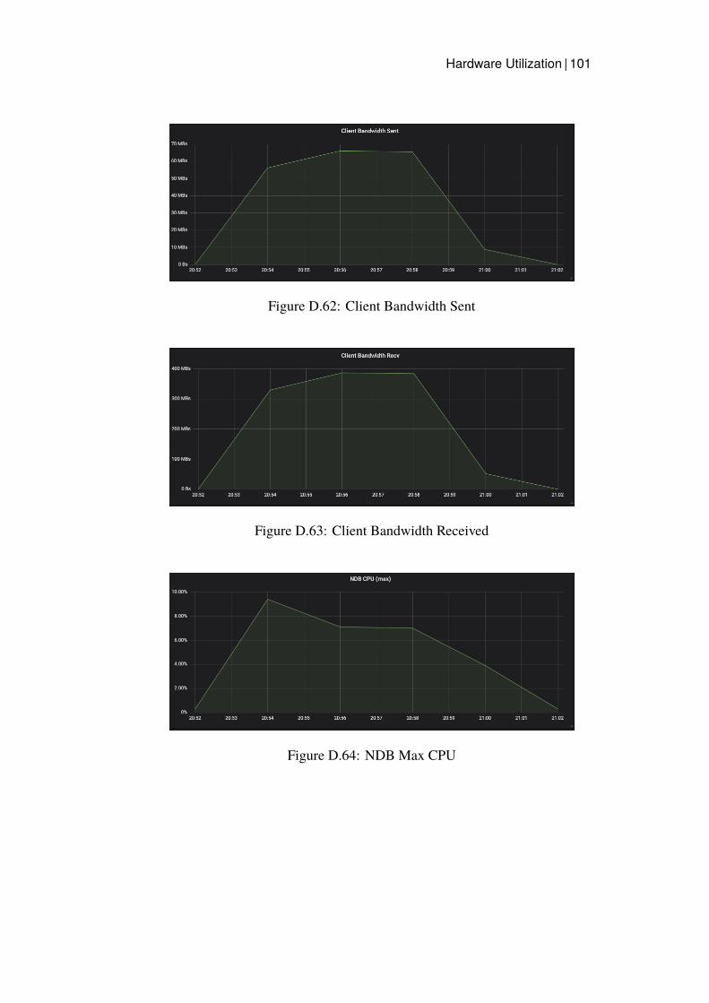
Hardware Utilization | 101
Figure D.62: Client Bandwidth Sent
Figure D.63: Client Bandwidth Received
Figure D.64: NDB Max CPU
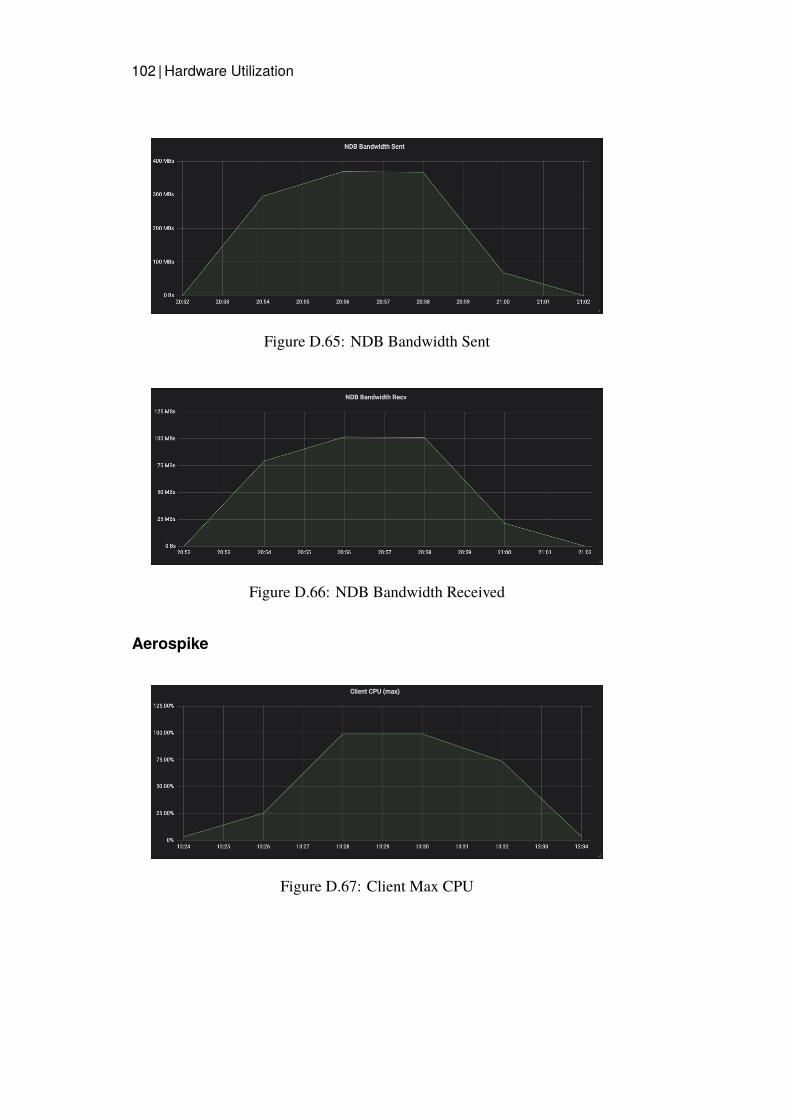
102 |Hardware Utilization
Figure D.65: NDB Bandwidth Sent
Figure D.66: NDB Bandwidth Received
Aerospike
Figure D.67: Client Max CPU

Hardware Utilization | 103
Figure D.68: Client Bandwidth Sent
Figure D.69: Client Bandwidth Received
Figure D.70: Aerospike Max CPU

104 |Hardware Utilization
Figure D.71: Aerospike Bandwidth Sent
Figure D.72: Aerospike Bandwidth Received
D.1.7 2 Clients, 6 Nodes & 16 Threads
NDB
Figure D.73: Client Max CPU

Hardware Utilization | 105
Figure D.74: Client Bandwidth Sent
Figure D.75: Client Bandwidth Received
Figure D.76: NDB Max CPU

106 |Hardware Utilization
Figure D.77: NDB Bandwidth Sent
Figure D.78: NDB Bandwidth Received
Aerospike
Figure D.79: Client Max CPU

Hardware Utilization | 107
Figure D.80: Client Bandwidth Sent
Figure D.81: Client Bandwidth Received
Figure D.82: Aerospike Max CPU

108 |Hardware Utilization
Figure D.83: Aerospike Bandwidth Sent
Figure D.84: Aerospike Bandwidth Received
D.1.8 2 Clients, 6 Nodes & 32 Threads
Aerospike
Figure D.85: Client Max CPU

Hardware Utilization | 109
Figure D.86: Client Bandwidth Sent
Figure D.87: Client Bandwidth Received
Figure D.88: Aerospike Max CPU

110 |Hardware Utilization
Figure D.89: Aerospike Bandwidth Sent
Figure D.90: Aerospike Bandwidth Received
D.1.9 4 Clients, 6 Nodes & 16 Threads
NDB
Figure D.91: Client Max CPU

Hardware Utilization | 111
Figure D.92: Client Bandwidth Sent
Figure D.93: Client Bandwidth Received
Figure D.94: NDB Max CPU

112 |Hardware Utilization
Figure D.95: NDB Bandwidth Sent
Figure D.96: NDB Bandwidth Received
Aerospike
Figure D.97: Client Max CPU

Hardware Utilization | 113
Figure D.98: Client Bandwidth Sent
Figure D.99: Client Bandwidth Received
Figure D.100: Aerospike Max CPU

114 |Hardware Utilization
Figure D.101: Aerospike Bandwidth Sent
Figure D.102: Aerospike Bandwidth Received
D.1.10 8 Clients, 6 Nodes & 16 Threads
NDB
Figure D.103: Client Max CPU

Hardware Utilization | 115
Figure D.104: Client Bandwidth Sent
Figure D.105: Client Bandwidth Received
Figure D.106: NDB Max CPU

116 |Hardware Utilization
Figure D.107: NDB Bandwidth Sent
Figure D.108: NDB Bandwidth Received
NDB without Spinning
Figure D.109: Client Max CPU

Hardware Utilization | 117
Figure D.110: Client Bandwidth Sent
Figure D.111: Client Bandwidth Received
Figure D.112: NDB Max CPU

118 |Hardware Utilization
Figure D.113: NDB Bandwidth Sent
Figure D.114: NDB Bandwidth Received
Aerospike
Figure D.115: Client Max CPU

Hardware Utilization | 119
Figure D.116: Client Bandwidth Sent
Figure D.117: Client Bandwidth Received
Figure D.118: Aerospike Max CPU

120 |Hardware Utilization
Figure D.119: Aerospike Bandwidth Sent
Figure D.120: Aerospike Bandwidth Received
D.1.11 1 Client, 8 Nodes & 1 Thread
NDB
Figure D.121: Client Max CPU

Hardware Utilization | 121
Figure D.122: Client Bandwidth Sent
Figure D.123: Client Bandwidth Received
Figure D.124: NDB Max CPU

122 |Hardware Utilization
Figure D.125: NDB Bandwidth Sent
Figure D.126: NDB Bandwidth Received
Aerospike
Figure D.127: Client Max CPU

Hardware Utilization | 123
Figure D.128: Client Bandwidth Sent
Figure D.129: Client Bandwidth Received
Figure D.130: Aerospike Max CPU

124 |Hardware Utilization
Figure D.131: Aerospike Bandwidth Sent
Figure D.132: Aerospike Bandwidth Received
D.1.12 1 Client, 8 Nodes & 2 Threads
NDB
Figure D.133: Client Max CPU

Hardware Utilization | 125
Figure D.134: Client Bandwidth Sent
Figure D.135: Client Bandwidth Received
Figure D.136: NDB Max CPU

126 |Hardware Utilization
Figure D.137: NDB Bandwidth Sent
Figure D.138: NDB Bandwidth Received
Aerospike
Figure D.139: Client Max CPU

Hardware Utilization | 127
Figure D.140: Client Bandwidth Sent
Figure D.141: Client Bandwidth Received
Figure D.142: Aerospike Max CPU

128 |Hardware Utilization
Figure D.143: Aerospike Bandwidth Sent
Figure D.144: Aerospike Bandwidth Received
D.1.13 1 Client, 8 Nodes & 4 Threads
NDB
Figure D.145: Client Max CPU
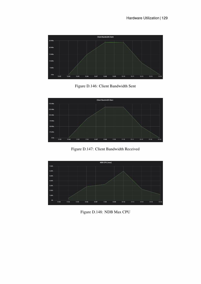
Hardware Utilization | 129
Figure D.146: Client Bandwidth Sent
Figure D.147: Client Bandwidth Received
Figure D.148: NDB Max CPU

130 |Hardware Utilization
Figure D.149: NDB Bandwidth Sent
Figure D.150: NDB Bandwidth Received
Aerospike
Figure D.151: Client Max CPU

Hardware Utilization | 131
Figure D.152: Client Bandwidth Sent
Figure D.153: Client Bandwidth Received
Figure D.154: Aerospike Max CPU

132 |Hardware Utilization
Figure D.155: Aerospike Bandwidth Sent
Figure D.156: Aerospike Bandwidth Received
D.1.14 1 Client, 8 Nodes & 8 Threads
NDB
Figure D.157: Client Max CPU

Hardware Utilization | 133
Figure D.158: Client Bandwidth Sent
Figure D.159: Client Bandwidth Received
Figure D.160: NDB Max CPU

134 |Hardware Utilization
Figure D.161: NDB Bandwidth Sent
Figure D.162: NDB Bandwidth Received
Aerospike
Figure D.163: Client Max CPU

Hardware Utilization | 135
Figure D.164: Client Bandwidth Sent
Figure D.165: Client Bandwidth Received
Figure D.166: Aerospike Max CPU

136 |Hardware Utilization
Figure D.167: Aerospike Bandwidth Sent
Figure D.168: Aerospike Bandwidth Received
D.1.15 1 Client, 8 Nodes & 16 Threads
NDB
Figure D.169: Client Max CPU

Hardware Utilization | 137
Figure D.170: Client Bandwidth Sent
Figure D.171: Client Bandwidth Received
Figure D.172: NDB Max CPU

138 |Hardware Utilization
Figure D.173: NDB Bandwidth Sent
Figure D.174: NDB Bandwidth Received
Aerospike
Figure D.175: Client Max CPU

Hardware Utilization | 139
Figure D.176: Client Bandwidth Sent
Figure D.177: Client Bandwidth Received
Figure D.178: Aerospike Max CPU

140 |Hardware Utilization
Figure D.179: Aerospike Bandwidth Sent
Figure D.180: Aerospike Bandwidth Received
D.1.16 1 Client, 8 Nodes & 32 Threads
NDB
Figure D.181: Client Max CPU

Hardware Utilization | 141
Figure D.182: Client Bandwidth Sent
Figure D.183: Client Bandwidth Received
Figure D.184: NDB Max CPU

142 |Hardware Utilization
Figure D.185: NDB Bandwidth Sent
Figure D.186: NDB Bandwidth Received
Aerospike
Figure D.187: Client Max CPU

Hardware Utilization | 143
Figure D.188: Client Bandwidth Sent
Figure D.189: Client Bandwidth Received
Figure D.190: Aerospike Max CPU

144 |Hardware Utilization
Figure D.191: Aerospike Bandwidth Sent
Figure D.192: Aerospike Bandwidth Received
D.1.17 2 Clients, 8 Nodes & 16 Threads
NDB
Figure D.193: Client Max CPU
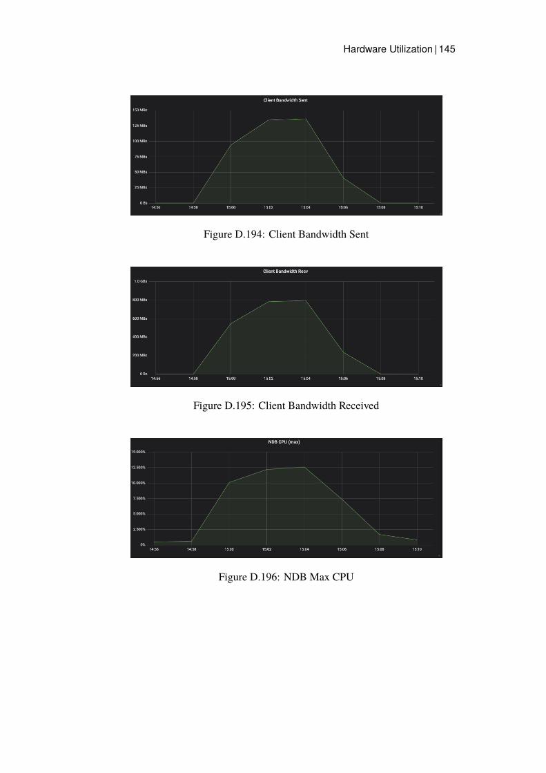
Hardware Utilization | 145
Figure D.194: Client Bandwidth Sent
Figure D.195: Client Bandwidth Received
Figure D.196: NDB Max CPU

146 |Hardware Utilization
Figure D.197: NDB Bandwidth Sent
Figure D.198: NDB Bandwidth Received
Aerospike
Figure D.199: Client Max CPU

Hardware Utilization | 147
Figure D.200: Client Bandwidth Sent
Figure D.201: Client Bandwidth Received
Figure D.202: Aerospike Max CPU

148 |Hardware Utilization
Figure D.203: Aerospike Bandwidth Sent
Figure D.204: Aerospike Bandwidth Received
D.1.18 4 Clients, 8 Nodes & 16 Threads
NDB
Figure D.205: Client Max CPU

Hardware Utilization | 149
Figure D.206: Client Bandwidth Sent
Figure D.207: Client Bandwidth Received
Figure D.208: NDB Max CPU

150 |Hardware Utilization
Figure D.209: NDB Bandwidth Sent
Figure D.210: NDB Bandwidth Received
Aerospike
Figure D.211: Client Max CPU

Hardware Utilization | 151
Figure D.212: Client Bandwidth Sent
Figure D.213: Client Bandwidth Received
Figure D.214: Aerospike Max CPU

152 |Hardware Utilization
Figure D.215: Aerospike Bandwidth Sent
Figure D.216: Aerospike Bandwidth Received
D.1.19 8 Clients, 8 Nodes & 16 Threads
NDB
Figure D.217: Client Max CPU

Hardware Utilization | 153
Figure D.218: Client Bandwidth Sent
Figure D.219: Client Bandwidth Received
Figure D.220: NDB Max CPU

154 |Hardware Utilization
Figure D.221: NDB Bandwidth Sent
Figure D.222: NDB Bandwidth Received
Aerospike
Figure D.223: Client Max CPU

Hardware Utilization | 155
Figure D.224: Client Bandwidth Sent
Figure D.225: Client Bandwidth Received
Figure D.226: Aerospike Max CPU

156 |Hardware Utilization
Figure D.227: Aerospike Bandwidth Sent
Figure D.228: Aerospike Bandwidth Received

Hardware Utilization | 157
D.2 Write Program
D.2.1 6 Nodes & 128 workers
Aerospike
Figure D.229: Aerospike Max CPU
Figure D.230: Aerospike Max Disk IO
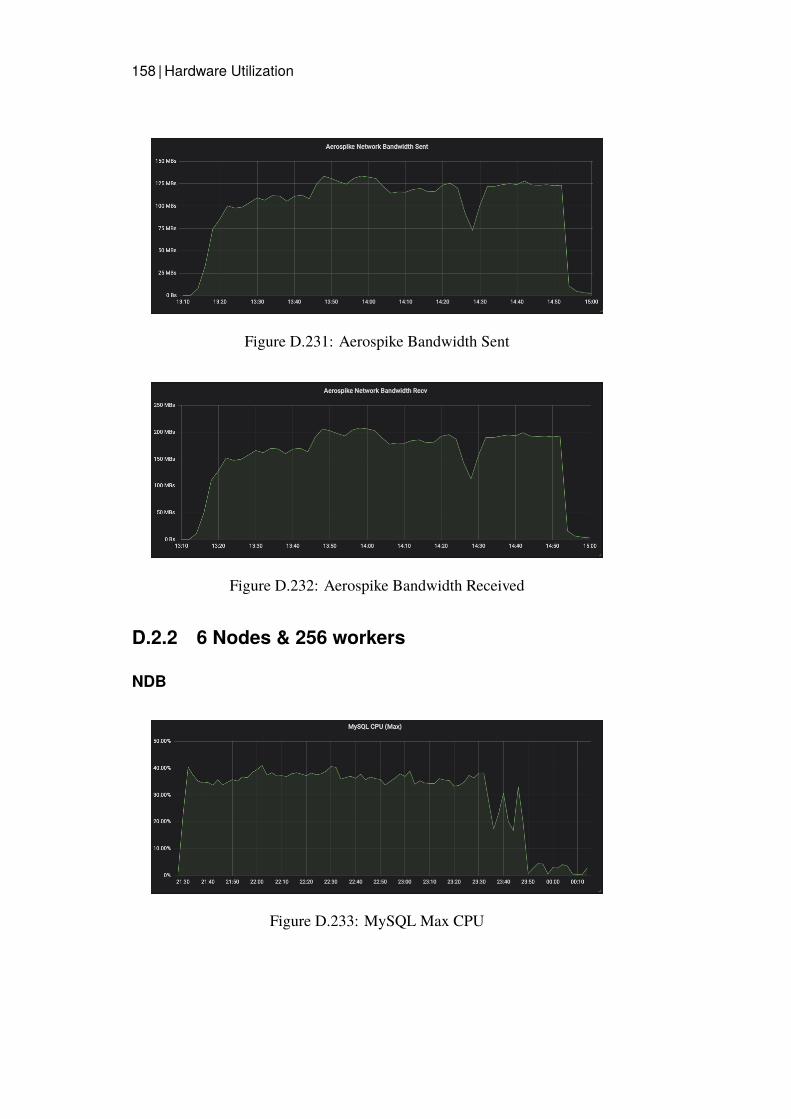
158 |Hardware Utilization
Figure D.231: Aerospike Bandwidth Sent
Figure D.232: Aerospike Bandwidth Received
D.2.2 6 Nodes & 256 workers
NDB
Figure D.233: MySQL Max CPU

Hardware Utilization | 159
Figure D.234: MySQL Bandwidth Sent
Figure D.235: MySQL Bandwidth Received
Figure D.236: NDB Max CPU

160 |Hardware Utilization
Figure D.237: NDB Max Disk IO
Figure D.238: NDB Bandwidth Sent
Figure D.239: NDB Bandwidth Received

Hardware Utilization | 161
Aerospike
Figure D.240: Aerospike Max CPU
Figure D.241: Aerospike Max Disk IO
Figure D.242: Aerospike Bandwidth Sent

162 |Hardware Utilization
Figure D.243: Aerospike Bandwidth Received
D.2.3 6 Nodes & 512 workers
NDB
Figure D.244: MySQL Max CPU
Figure D.245: MySQL Bandwidth Sent

Hardware Utilization | 163
Figure D.246: MySQL Bandwidth Received
Figure D.247: NDB Max CPU
Figure D.248: NDB Max Disk IO

164 |Hardware Utilization
Figure D.249: NDB Bandwidth Sent
Figure D.250: NDB Bandwidth Received
Aerospike
Figure D.251: Aerospike Max CPU

Hardware Utilization | 165
Figure D.252: Aerospike Max Disk IO
Figure D.253: Aerospike Bandwidth Sent
Figure D.254: Aerospike Bandwidth Received

166 |Hardware Utilization
D.2.4 8 Nodes & 256 Workers
NDB
Figure D.255: MySQL Max CPU
Figure D.256: MySQL Bandwidth Sent
Figure D.257: MySQL Bandwidth Received

Hardware Utilization | 167
Figure D.258: NDB Max CPU
Figure D.259: NDB Max Disk IO
Figure D.260: NDB Bandwidth Sent
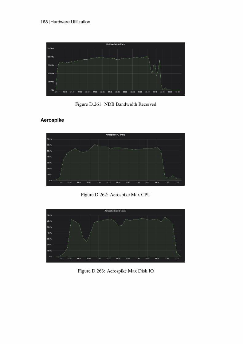
168 |Hardware Utilization
Figure D.261: NDB Bandwidth Received
Aerospike
Figure D.262: Aerospike Max CPU
Figure D.263: Aerospike Max Disk IO

Hardware Utilization | 169
Figure D.264: Aerospike Bandwidth Sent
Figure D.265: Aerospike Bandwidth Received
D.2.5 8 Nodes & 512 Workers
NDB
Figure D.266: MySQL Max CPU
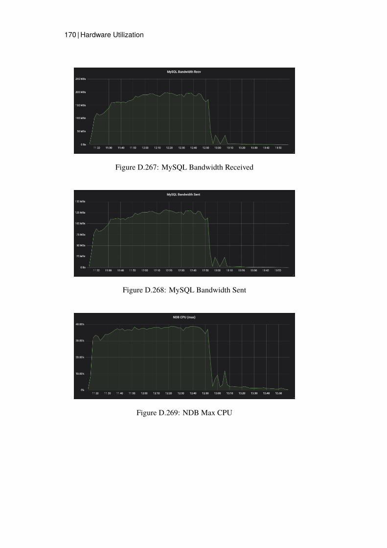
170 |Hardware Utilization
Figure D.267: MySQL Bandwidth Received
Figure D.268: MySQL Bandwidth Sent
Figure D.269: NDB Max CPU

Hardware Utilization | 171
Figure D.270: NDB Max Disk IO
Figure D.271: NDB Bandwidth Sent
Figure D.272: NDB Bandwidth Received

172 |Hardware Utilization
Aerospike
Figure D.273: Aerospike Max CPU
Figure D.274: Aerospike Max Disk IO
Figure D.275: Aerospike Bandwidth Sent

Hardware Utilization | 173
Figure D.276: Aerospike Bandwidth Received
D.3 Write & Read Benchmark
D.3.1 6 Nodes & 256 Workers
NDB
Figure D.277: Client Max CPU

174 |Hardware Utilization
Figure D.278: Client Bandwidth Sent
Figure D.279: Client Bandwidth Received
Figure D.280: MySQL Max CPU

Hardware Utilization | 175
Figure D.281: MySQL Bandwidth Sent
Figure D.282: MySQL Bandwidth Received
Figure D.283: NDB Max CPU

176 |Hardware Utilization
Figure D.284: NDB Max Disk IO
Figure D.285: NDB Bandwidth Sent
Figure D.286: NDB Bandwidth Received

Hardware Utilization | 177
Aerospike
Figure D.287: Client Max CPU
Figure D.288: Client Bandwidth Sent
Figure D.289: Client Bandwidth Received

178 |Hardware Utilization
Figure D.290: Aerospike Max CPU
Figure D.291: Aerospike Max Disk IO
Figure D.292: Aerospike Bandwidth Sent

Hardware Utilization | 179
Figure D.293: Aerospike Bandwidth Received
D.3.2 6 Nodes & 512 Workers
NDB
Figure D.294: Client Max CPU
Figure D.295: Client Bandwidth Sent

180 |Hardware Utilization
Figure D.296: Client Bandwidth Received
Figure D.297: MySQL Max CPU
Figure D.298: MySQL Bandwidth Sent

Hardware Utilization | 181
Figure D.299: MySQL Bandwidth Received
Figure D.300: NDB Max CPU
Figure D.301: NDB Max Disk IO

182 |Hardware Utilization
Figure D.302: NDB Bandwidth Sent
Figure D.303: NDB Bandwidth Received
Aerospike
Figure D.304: Client Max CPU

Hardware Utilization | 183
Figure D.305: Client Bandwidth Sent
Figure D.306: Client Bandwidth Received
Figure D.307: Aerospike Max CPU

184 |Hardware Utilization
Figure D.308: Aerospike Max Disk IO
Figure D.309: Aerospike Bandwidth Sent
Figure D.310: Aerospike Bandwidth Received

Hardware Utilization | 185
D.3.3 8 Nodes & 256 Workers
NDB
Figure D.311: Client Max CPU
Figure D.312: Client Bandwidth Sent
Figure D.313: Client Bandwidth Received

186 |Hardware Utilization
Figure D.314: MySQL Max CPU
Figure D.315: MySQL Bandwidth Sent
Figure D.316: MySQL Bandwidth Received
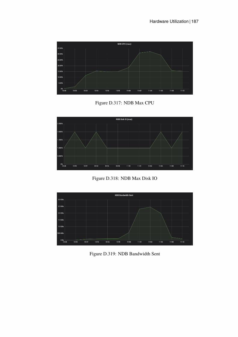
Hardware Utilization | 187
Figure D.317: NDB Max CPU
Figure D.318: NDB Max Disk IO
Figure D.319: NDB Bandwidth Sent

188 |Hardware Utilization
Figure D.320: NDB Bandwidth Received
Aerospike
Figure D.321: Client Max CPU
Figure D.322: Client Bandwidth Sent
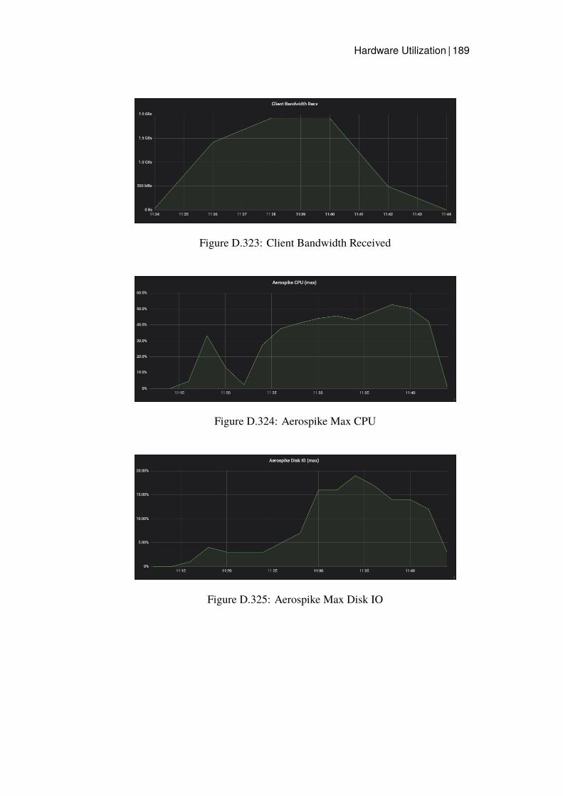
Hardware Utilization | 189
Figure D.323: Client Bandwidth Received
Figure D.324: Aerospike Max CPU
Figure D.325: Aerospike Max Disk IO

190 |Hardware Utilization
Figure D.326: Aerospike Bandwidth Sent
Figure D.327: Aerospike Bandwidth Received
D.3.4 8 Nodes & 512 Workers
NDB
Figure D.328: Client Max CPU

Hardware Utilization | 191
Figure D.329: Client Bandwidth Sent
Figure D.330: Client Bandwidth Received
Figure D.331: MySQL Max CPU
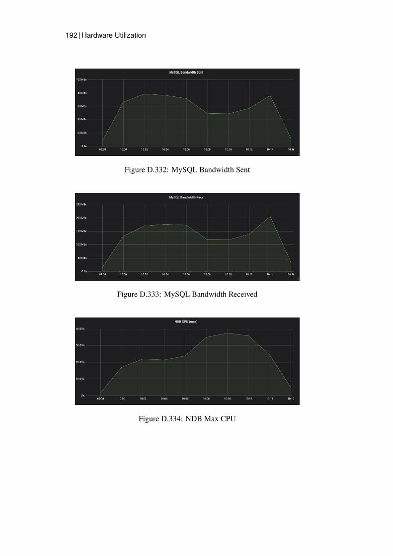
192 |Hardware Utilization
Figure D.332: MySQL Bandwidth Sent
Figure D.333: MySQL Bandwidth Received
Figure D.334: NDB Max CPU

Hardware Utilization | 193
Figure D.335: NDB Max Disk IO
Figure D.336: NDB Bandwidth Sent
Figure D.337: NDB Bandwidth Received

194 |Hardware Utilization
Aerospike
Figure D.338: Client Max CPU
Figure D.339: Client Bandwidth Sent
Figure D.340: Client Bandwidth Received

Hardware Utilization | 195
Figure D.341: Aerospike Max CPU
Figure D.342: Aerospike Max Disk IO
Figure D.343: Aerospike Bandwidth Sent

196 |Hardware Utilization
Figure D.344: Aerospike Bandwidth Received

For DIVA
{"Author1": { "name": "Alexander Volminger"},"Degree": {"Educational program": "Civilingenjör Datateknik"},"Title": {"Main title": "A comparison of Data Stores for the Online Feature Store Component","Subtitle": "A comparison between NDB and Aerospike","Language": "eng" },"Alternative title": {"Main title": "En jämförelse av datalagringssystem för andvänding som Online Feature Store","Subtitle": "En jämförelse mellan NDB och Aerospike","Language": "swe"},"Supervisor1": { "name": "Jim Dowling" },"Examiner": {"name": "Stefano Markidis","organisation": {"L1": "School of Electrical Engineering and Computer Science" }},"Cooperation": { "Partner_name": "Spotify AB"},"Other information": {"Year": "2021", "Number of pages": "x,56"}}

TRITA-EECS-EX-2021:132
www.kth.se