2016

The Western Undergraduate Economics Review is an annual publication containing papers written by undergraduate students in Economics at Western. First published in 2002, the Review reflects the academic distinction and creativity of the Economics Department at Western. By showcasing some of the finest work of our students, it bestows on them a lasting honour and a sense of pride. Moreover, publication in the Review is highly beneficial to the students as they continue their studies or pursue other activities after graduation. For many, it is their first publication, and the experience of becoming a published author is a highlight of their undergraduate career. The Review is a collaborative effort of the students, faculty, and staff of the Economics Department. All papers submitted to the Review are essays written for courses taken in the Department. Some are by students in the early stages of their Economics studies, while others are papers written by senior students for the Department’s unique thesis course, Economics 4400. Selections are made by the edition editors, in consultation with a faculty advisor, based on creativity, academic merit, and the written quality of the article. Editors Mitchell Nicholson Yan Wang Faculty Advisor Administrative Support Tai-Yeong Chung Leslie Kostal © The Western Undergraduate Economic Review (WUER) is published by the Department of Economics, Faculty of Social Science, Western University, London, ON Canada N6A 5C2. For submission information, please visit the WUER website. http://economics.uwo.ca/undergraduate/undergraduate_economics_review.html

ISSN 1705-6098

ii

Editors’ Comments ....................................................................................... iii Does Gender Inequality Within a Country Increase the Burden of HIV on Females?

Victoria Turner ............................................................................................. 1 Winner of the Mark K. Inman Senior Essay Prize, 2015 An Assessment of the Effect of Ageing Populations on Interest Rates in OECD Countries Anushay Wahab and Audrey Au Yong Lyn .................................................. 23 How Does Information and Communication Technology Influence Agricultural Development: Evidence from China Fan Yang and Peidong Wang ...................................................................... 48 The Wealth Effects of Stock Market on Consumption: A Time-Series Analysis of the US from 1952 to 2014 Renjie Wang ................................................................................................ 64

iii

The 2016 edition of the Western Undergraduate Economics Review (WUER) showcases the diversity of high quality research completed by Western’s Undergraduate Economics students. This year, the Review includes a collection of papers that provide pertinent conclusions for economic policy in the United States and China, as well as policies that target important social groups such as women and the ageing population. Together, these results highlight the global perspective that is at the core of economics at Western. This Review begins with an outstanding contribution made by Victoria Turner, who was the winner of the Mark K. Inman Senior Essay Prize and also the previous Senior Editor of the WUER. Turner evaluated the effect of gender equality on the burden of HIV on females, which ultimately proved to be an empowering work for addressing gender disparities in developing countries. This paper is followed by a second senior thesis written by Anushay Wahab and Audrey Au Yong Lyn, on the effect of an ageing population on interest rates in OECD countries. Wahab and Lyn's paper is very relevant when one considers the ageing of the baby-boomer generation, in conjunction with low interest rates that prevail in the current global economy. The third paper in this edition is another excellent example of the work completed in the senior thesis course. Fan Yang and Peidong Wang's contribution analyzes influence information and communication technology on agricultural development in China. Lastly, Renjie Wang wrote a detailed paper on the wealth effect of the stock market on consumption in the United States and employs strong empirical techniques to determine his results. We hope that you enjoy reading the 2016 edition of the Western Economics Undergraduate Review and also gain a deeper appreciation for the quality of undergraduate economic research conducted at Western. Further, we would like to thank each of the authors for their contribution to this year's excellent edition of the WUER and we hope this edition inspires future economics students at Western to work even more diligently at their research. Mitchell Nicholson Yan Wang London, Ontario April 2016

Acknowledgments

We also extend our sincere thanks to the Social Science Student Donation Fund for its ongoing financial support of the Western Undergraduate Economics Review.

1

Abstract

This paper evaluates the claim that the persistent burden of HIV/AIDS on females in developing countries is caused by gender inequality within those countries using OLS regression. Previous economic literature explores behavioural change in the face of HIV/AIDS, and how gender inequality may hinder the ability of females to decrease their risk. This paper deviates from previous work through both the variables used and the analysis provided, with the most lasting contribution likely being the use and analysis of the “Social Institutions & Gender Index” (SIGI) as a measure of gender inequality, particularly for low-development regions. The SIGI uniquely captures country-specific factors that should directly impact a woman’s “intra-household bargaining power”: a potential mechanism for a causal relationship between gender inequality and the HIV/AIDS burden on females. The results of this study not only provide support for the use of the SIGI as a measure of bargaining power, but also evidence that gender inequality is contributing to HIV/AIDS in female populations in some regions.

Acknowledgments I would like to thank Professors Chung, Robinson and Sicular for their constant guidance and support that has allowed me to complete this paper. Many thanks are also owed to Mr. Vince Gray for his dedication in helping me locate the specific data I required, as well as the class of 4400E and our teaching assistant Antonella Mancino for their helpful feedback and assistance. Introduction HIV/AIDS has taken many lives worldwide since its first appearance in human populations. In more recent years, however, The HIV/AIDS epidemic in developed countries represents a great victory of both the medical and political/social communities, as this a disease whose spread was contained through advancements in understanding the disease and medical treatments, as well as educating the public on how to drastically reduce risk of obtaining HIV/AIDS. In developed countries such as the United States, the persisting HIV/AIDS epidemic is heavily concentrated in specific groups such as men who have sex with men, intravenous drug users, and African Americans due to both the mechanisms of HIV transmission and racial health inequities (CDC, 2014). In developing nations, however, the aforementioned “victory” is far from being realized, with large numbers of the population still being affected by this disease, across all demographics. In

2

Sub-Saharan Africa, for example, where the AIDS epidemic is still extremely severe, 58 percent of HIV-positive adults are women (WHO, 2003). This lies in stark contrast to the small proportion of women in the U.S. making up new HIV infections, as demonstrated by Figure 1 in the Appendix. Despite the fact that countries with high socio-economic development have very low prevalence and incidence of HIV/AIDS in the female demographic, UNAIDS has identified females as a target group being “left behind” in the gains being made in combatting the HIV/AIDS epidemic (UNAIDS, 2014). Increasing or even stagnant rates of HIV transmission in females is concerning for two reasons: first, heterosexual transmission of the virus is far less likely than other methods such as homosexual intercourse and through intravenous drugs, and secondly because HIV/AIDS is a disease whose risks are very easily mitigated through fairly simple actions. The data on persistent HIV transmission rates in women suggest that women are not taking enough action or precaution to reduce their risk of infection. This thesis seeks to test the sociological theory that these persistent gender differences in HIV/AIDS “…stem from…socially constructed ‘gender’ differences between women and men in roles and responsibilities, access to resources and decision-making power” (Tsafack Temah, 2008) under an economic framework. The theoretical aspect of my study is based on the idea of intra-household bargaining, and how measures of gender inequality for a particular region can reduce the bargaining power of women in marital and non-marital relationships. This theoretical background provides the justification for a potential causal relationship between a measure of gender inequality for a country and the ratio of female to male incidence rate (defined as the number of new cases per 100,000 people in a given year) within that country. The use of incidence over prevalence1, is a deliberate choice as this allows us to observe the number of females that have newly acquired the virus, in an environment where individuals largely know the mechanisms of the disease, the prevalence of the disease in their society, and ways to reduce their risk. The use of incidence as the dependent variable, as well as employing the new and unique “Social Institutions & Gender Index” as the key independent variable, representing gender inequality and female bargaining power, differentiate my work from previous empirical studies on this issue. The following paper begins by outlining the economic intuition and past work motivating the economic analysis of HIV/AIDS, with a particular focus on the impact of gender inequality on HIV/AIDS under an economic framework. After the framework is set out, there will be a description of the methods employed and the data used in the empirical component of this study. Finally, results of the empirical study are presented and analyzed, and conclusions are drawn.

1Prevalence is used as the dependent variable in many economic studies on HIV/AIDS such as “Gender Inequality and the HIV/AIDS Epidemic in Sub-Saharan Africa” (Tsafack Temah, 2008).

3

1. Literature Review and Theoretical Background HIV/AIDS in Existing Literature

Many economists have attempted to understand realities of the HIV/AIDS epidemic under a framework of microeconomics, and rational individuals making choices in response to existing conditions. Philipson and Posner (1993) focused on the risks that AIDS posed to American society at the time. They referenced a poignant shift in behaviour (from risky to safer) in homosexuals and intravenous drug users in response to the AIDS threat as a justification for using economics to analyze the spread and combatting of HIV/AIDS (Philipson and Posner, 1993, 68). The observed reduction in infection rates of both HIV/AIDS and other STI’s in homosexuals at this time in addition to survey data on sexual practices demonstrates that increased prevalence of HIV (and therefore higher costs of unsafe sex), lead to a shift away from risky sex (Philipson and Posner, 1993, 69). This provides some empirical justification for the microeconomic analysis of HIV/AIDS as being useful. Philipson and Posner (1995) also addressed the differences between the transmission of HIV/AIDS in developed countries and in developing countries (particularly those in sub-Saharan Africa). This paper proposes some issues specific to Sub-Saharan Africa that provide an economic explanation for the lack of behavioural changes made in response to high HIV prevalence in this region. These issues include a lack of education that decrease perceived costs of risky behaviours and benefits of safe behaviours, lower life expectancy which decreases cost of acquiring HIV/AIDS (and thus lowers cost of risky sex), and higher cost of safe practices such as condoms (Philipson and Posner, 1995, 840). In this paper, Philipson and Posner also introduced the issue of gender differences, and how unusually in Sub-Saharan Africa women’s prevalence of the disease is equal to that of men, and that the predominant mode of transmission tends to be heterosexual intercourse, as opposed to homosexual intercourse and injected drug use as in the US and other developed countries (Philipson and Posner, 1995, 842). Philipson and Posner briefly discuss their intuition that these differences can largely be explained by gender inequality due to the fact that higher gender inequality increases the likelihood of women turning to sex work as they have few labour market opportunities, and also lowers their ability to negotiate safe sex practices (Philipson and Posner, 1995, 844). These issues are discussed in other economic literature related to HIV/AIDS with regards to other social issues, which I will address in the next section. Gaffeo (2003) also provides some motivation for a microeconomic analysis of HIV/AIDS economics, as it provides a useful framework for analyzing the continued spread of the disease under “market failures.” Gaffeo importantly introduces the externalities posed by the institution of marriage in many developing countries (Gaffeo, 2003, 31). The inability of women to be granted divorce, for example, reduces their ability to react to change in incentives for pursuing safe sex. If they suspect their husband of having extra marital relations for example, there is little they can do to demand safer sex or even to reject intercourse, as they do not have the ability to leave the marriage if their demands are not met.

4

Theoretically, economics can demonstrate how there may be a causal link between gender inequality and HIV/AIDS rates, particularly in some regions of the world. To demonstrate this concept empirically, however, can be difficult and thus there is less literature that presents empirical analysis. Richardson et al. (2014), motivates my work in that this study is a cross-country empirical analysis of the impact of gender inequality on HIV transmission. However, the variables used are very different from the methods I employ. Richardson et al.’s (2014) paper is interested in determining how gender inequality is related to the primary mode of HIV transmission within in a country: namely whether or not an epidemic is primarily driven by transmission through heterosexual transmission, or men who have sex with men and intravenous drug use transmission (Richardson et al., 2014). This paper is limited to low development areas, where the vast majority of epidemics are driven by heterosexual transmission, and instead explores the relationship between gender inequality differences in developing nations and the female to male ratio of HIV incidence. Tsafack Temah’s (2008) earlier draft, “Socio-Economic Inequalities and HIV/AIDS Epidemic: Evidence from Sub-Saharan Africa” evaluates how both economic and gender inequalities are related to HIV prevalence within a country. Tsafack Temah (2008) uses a variety of variables that measure gender inequality as independent variables such as female estimated earned income and percentage of women in the labor force, instead of a single index (Tsafack Temah, 2008). The significance of employing the Social Institutions & Gender Index in this study is to evaluate entrenched social norms and institutions as a measure of bargaining power, and determine this effect on HIV/AIDS gender ratios. These previous works of literature demonstrate how emerging gender disparities in the HIV/AIDS epidemic can be explained through economic concepts. Another crucial economic concept in analyzing this issue under an economic framework is bargaining power, particularly intra-household bargaining power, which allows us to understand how different variables affect an individual’s decision-making power within relationships. This is important in analyzing the impact of gender inequality on the gender disparities within HIV/AIDS incidence because in countries where women have little social and economic power, their power to make meaningful decisions about both their sexual activity and their health (both key determinants of HIV transmission) can be reduced. Theoretical Considerations

The concept of intra-household bargaining provides the key motivation for my research, and thus it is important to define what this means. Intra-household bargaining represents the move away from viewing household and marital decisions under a unitary model and single set of preferences. Instead, intra-household bargaining allows us to view individuals within a relationship or household as possessing competing preferences that require bargaining among the parties to achieve cooperative or non-cooperative solutions. As outlined in Katz (1997), each individual has some ability to bargain (or exercise “voice”) over household decisions (Katz, 1997, 32). At least under the cooperative view, this ability is largely decided by the individual’s “threat” or “fall-back” position, typically seen as their ability to “exit” the household. This position is largely impacted by social conditions, Katz argues, such as the view of divorced women in

5

society and their ability to earn income outside of marriage. This is important to the impact of gender inequality on HIV/AIDS, as bargaining can also be applied to sexual decisions. In the view of marriage, the prevalence of extra-marital affairs by males in gender-unequal societies places females at risk due to their inability to bargain safer sex with their husbands. Additionally, the model can be applied to non-married partners, in my opinion, more accurately under a non-cooperative model.

Luke (2005) provides some insight into the market for sex in Sub-Saharan Africa, and its implications for HIV/AIDS transmission. This paper discusses the idea of “sugar daddy” relationships, in which young women engage in sexual relationships with older more wealthy men, and a key part of this relationship entails transfer of resources from the male to female (Luke, 2005, 6). While this is not quite a case of prostitution, and likely the female is not solely dependent on the sugar daddy for income, the degree to which she relies on the transfer of resources can greatly reduce her ability to bargain safe sex practices. Luke (2005) points to the shift of resources away from females in developing countries (both from parents and the labour market), low education, and high ratio of young females as a reason for the dependence on these sorts of relationships.

This type of relationship tends to follow the “conjugal contract” model as outlined in sources such as Alderman et al. (1995). This more non-cooperative model views the household participants as having their own income to spend, yet one partner makes transfers to the other as a result of bargaining. This can be clearly applied to marriage but also transactional sexual relationships. Part of this negotiable transfer can also be seen as safe sex practices such as condom use and sexual exclusivity. Once again, bargaining over this transferable income or resources is dependent on the threat point of the women either as divorce, or ending the sexual relationship which in turn depends on sex ratios, dissolution of marriage laws, labour opportunities for females, etc.

Typically, empirical work regarding intra-household bargaining power looks at how changing variables of households affects outcomes within those households. For example, how mother’s education may impact outcomes within the household such as child health, or outcomes for the female children1. My thesis is largely differentiated from many of these works because I do not seek to examine the impact of a changing variable such as income or education on a specific outcome, but instead am motivated by the possibility of how social realities within a country effect the bargaining power of all women within that country to achieve safer sexual practices and sexual health. Mabsout and van Staveren (2005) provided some insight into how bargaining power of women can be greatly impacted by institutions. I use information from this paper in my analysis of how aspects of a country’s institutions, laws and customs impact overall bargaining power of the women within that country, which can translate to a disproportionately high amount of new cases of HIV (HIV/AIDS incidence for females).

1 i.e. Maiga, Eugnenie WH. The Impact of Mother’s Education on Child Health and Nutrition in Developing Countries: Evidence from a Natural Experiement in Burkina Faso. African Center for Economic Transformation (October 2011).

6

2. Empirical Methodology and Data Data and Variables

Table 2 in the Appendix provides a detailed description of the variables

considered, and those eventually used in the final model.

In order to effectively test whether or not the bargaining power of women has an impact on the gender ratios of HIV/AIDS incidence, it is important that my key independent variable is a proxy for gender inequality that incorporates those institutions, laws and customs that are likely to impact overall bargaining power of women. The “proxy” or index I have chosen for my research is the “Social Institutions & Gender Index” (SIGI) created by the OECD (2014). Table 1 in the appendix reports all 5 of the SIGI indices, and why each factor is relevant to female bargaining power. The SIGI is compiled from an average of these five indices, with each country receiving a final index value between 0 and 1, with a value closer to 1 representing higher gender inequality, and thus less female bargaining power within relationships. The reason I chose this specific index is because it seeks to incorporate factors that measure systemic and institutional discrimination within countries, such as formal and informal laws, norms and practices, which are often hard to quantify (OECD Development, 2014). This index is heavily concentrated towards developing nations, which is reasonable for my research because gender disparities of HIV/AIDS incidence and prevalence, i.e. the “feminization” of HIV/AIDS is largely concentrated in low income, less development nations.

As mentioned previously, this study critically uses HIV incidence rate (new cases) data to generate the ratio of female to male incidence, the dependent variable. The source of these data is the Institute for Health Metrics and Evaluation (IMHE, 2014)). The IMHE uses The UNAIDS Spectrum Model to produce their estimates, the methodology of which is beyond the scope of this study (Murray, 2014). Both UNAIDS (2014) and, by extension, the Institute for Health Metrics and Evaluation (2014) are presenting estimates, as it would not be possible to determine the exact number of people living with HIV due to the fact that people often do not know this information themselves or will not share this information (UNAIDS, 2014). UNAIDS is confident in their estimates, which incorporate all country HIV data available, information from pregnant mothers, and information in key populations in areas where epidemics are concentrated, as well as including assumptions from experts and literature. These data are provided from 1990-2013, yet only the most recent year is used, as this is a cross-sectional, non-time varying study. IMHE (2014) estimates, again drawn from the UNAIDS Spectrum model (2014), are also used for HIV prevalence, which is used as an important independent variable expected to impact the ratio of female to male HIV Incidence.

Outside of the key variables that represent the relationship between gender inequality (Bargaining power of women measured by the SIGI) and the burden of HIV on females (sex ratio of HIV Incidence measured by the IMHE data), there were many other variables considered that may also have an impact on the dependent variable. In the

7

section on “Methodology”, an exploration into the other independent variables that were considered and eventually chosen to model this relationship will be provided.

Evolution of Model

HIV/AIDS is clearly a very complex disease, and epidemics in different regions

are influenced by both the scientific and social realities of the specific area. The first area in which my model has evolved from the beginning of this undertaking to the final product is through the form of the dependent variable. My initial research plan outlined that I would evaluate the relationship between gender inequality and HIV/AIDS through regressing Female HIV Incidence on a measure of gender inequality, highly related to the bargaining power of women, and then using a regression with the Male HIV Incidence as an imperfect control. As my research unfolded it became clear that a more feasible dependent variable would be a generated ratio between the females and males. Since the data I acquired was a cross section of countries, the variation between the incidence rates of each observation was very large and clearly many factors would be involved in describing the cause of this variation. By using the ratio, the number of variables that would have to be included in the model to avoid large omitted variable bias can be drastically reduced, because now only variables that are likely to impact this gender disparity in HIV need to be included, as opposed to all factors related to both gender inequality and HIV rates.

The key independent variable, the SIGI, representing key components of intra-household bargaining power of women within a country, was also altered slightly from how I originally intended to use it. First, as previously mentioned the SIGI is largely skewed towards including low income, low development nations, as are the focus of this study. However, there are a few very highly developed countries whose results were included in the SIGI. Since higher development countries were not adequately represented, and the analysis of my paper is focused around developing countries and the nuances of the HIV epidemic specific to this type of region, I eliminated countries that are considered “very high development”, or within the top 50 ranking by the Human Development Index. Table 3 provides a list of countries initially provided by the SIGI, and highlights the countries that were dropped as a result of having a very high level of development.

Additionally, while I initially believed each of the five SIGI subindices adequately represented female bargaining power (higher score means higher inequality, and thus lower bargaining power), there is actually a valid economic argument for why one of the subindices has the opposite result on bargaining power. Subindex 3 represents “son bias”, demonstrating a preference for men in society, but also “missing women” suggesting that in countries where this value is high, there may be higher levels of infanticide, death by neglect, and abortion for female children. If there are more men in society, however, this can actually be equated with higher female bargaining power, particularly in sexual relationships, as the female can gain a new partner more easily. As a result, my final regression model generates a new variable as the index that represents female bargaining power (gender inequality) using only the other four SIGI subindices.

8

Methodology In order to determine the existence and magnitude of a relationship between

bargaining power in a country and the relative male and female HIV incidence, I regress the SIGI on the ratio of female HIV incidence (cases per 100,000 population) to male HIV incidence (cases per 100,000 population. As previously mentioned, a strong benefit of the SIGI is that the index is split into five distinct measures of discrimination/inequality, and thus I can also use the measure generated that discludes subindex 3, “Son Bias”, creating an even more accurate measure of female bargaining power. I believe the gender ratio of incidence is a good indicator because it demonstrates a “feminization” of HIV/AIDS incidence in the region if females are disproportionately represented in the new cases of HIV within a country. This analysis can provide a strong case for the global community to intervene in these types of systemic gender discrimination. I prefer incidence to prevalence because as demonstrated by the research of UNAIDS (2014) and other organizations, the emergence of higher prevalence of HIV in women is a more recent phenomenon with the gap between men and women narrowing in recent years (WHO, 2003). Prevalence measures include many people who were infected early in the epidemic when knowledge about the disease was low and the ability for individuals in developing countries to attempt to change their behaviour or the behaviour of their spouse/sexual partner was low. In today’s landscape, people even in the developing world are equipped with the knowledge and tools to protect themselves, and thus incidence rates increasing for females indicates that a market failure is occurring and that females are not taking an efficient level of precaution against this fatal disease. My hypothesis is that the SIGI, or more specifically the “new index” will be positively correlated with the gender incidence ratio, suggesting that gender discrimination that negatively impacts bargaining power may partially explain this market failure.

Clearly, the nuances of HIV/AIDS transmission are very complicated and dependent on both biological and social factors. Thus, I do not attempt to suggest that gender discrimination is the only factor contributing to a higher female incidence rate in many developing countries, but rather that it is one factor that can likely be addressed by global powers. In order to get an estimate with the least amount of bias, I must include other independent variables that are likely to impact the gender HIV/AIDS incidence ratio that are also expected to be correlated with the SIGI. I include HIV/AIDS prevalence, as Hertog (2008) describes why older, more established epidemics in the developing world are expected to tilt towards female incidence:

“In the early years of an epidemic driven by heterosexual transmission, HIV cases tend to be concentrated among female commercial sex workers and their clients such that male prevalence exceeds female prevalence. Over time, female prevalence increases as the wives and non-marital partners of those male clients become infected, eventually shifting the balance of HIV prevalence to women.” (Hertog, 2008, 3)

Prevalence works as a proxy for maturity of an epidemic as the longer an epidemic exists, the more people will be infected, particularly in the developing world where medical

9

breakthroughs have not had as much of an impact in curbing the epidemic. Prevalence is likely to be correlated with the SIGI as less developed countries tend to have less gender inequality as well as higher HIV prevalence.

In early regressions, I included GDP/capita as both gender equality and GDP per capita which are related to a country’s level of development. This tends to be correlated with HIV levels and transmission rates. On the advice of my peers I eventually decided to use GNI/Capita as a measure of economic development in the final regression: GNI/Capita includes only production within a country, and thus can more accurately gauge the standard of living of individuals within that country. GNI/capita is likely to have an impact on the HIV gender ratios in developing countries because in poor countries where living conditions are poor, people do not have the same access to resources that will allow them to gain information and methods of protecting themselves against HIV/AIDS. Particularly, women in poor countries tend to have an even more restricted access to resources. I previously considered other variables, namely health expenditure per capita and dummy variable for Muslim Majority that were likely to contribute to the female HIV incidence, but they were both statistically insignificant and lacked a significant theoretical basis to have an impact on the sex ratio of HIV incidence. Finally, I considered the use of other variables frequently used as indicators of female bargaining power or gender inequality that were not included in the SIGI, such as the estimated earned income of females as a percentage of males earned income. Interestingly, when I included the “earned income” variable in regression, the results were not significant. Malhotra and Mather (1997) find evidence from Sri Lanka that while factors such as a woman’s educational and employment history provide them greater negotiating power over household financial decisions, “domestic power on social and organizational issues may be embedded within more macro-level social institutions”( Malhotra and Mather, 1997, 626). In other words, when evaluating the impact of bargaining power on issues outside of financial decisions (such as money allocated to female children), including sexual decision-making, employment and educational factors of bargaining power may be less important than more institutionalized measures such as those included in the SIGI. As a result of the above discussion, the final empirical model is as follows:

[HIVincrat]=B0 + B1SIGI (original, and with dropped subindex 3) +

B2HIVprevalence + B3GNI/capita + e

Table 2 in the Appendix provides a detailed description of the variables. Once the regression results are presented, I assess both the economic and statistical significance of the key variables in order to draw conclusions.

10

3. Results and Discussion Results

The following presentation and analysis of results focuses on those results produced with the data that exclude highly developed regions, and the model presented in the previous section. Initial findings that were produced with the entire SIGI data set and alternative variables contributed significantly to this final model, and thus are presented and briefly explained in Appendix B: Initial Empirical Results.

As previously mentioned, my final model yields two separate regressions, one in which the key independent variable is the full Social Institutions & Gender Index, and one in which the key independent variable excludes the third subindex representing “Son Bias”. Results from the first regression, with the full index including subindex 3, are presented in Table 1. In this first regression, the key independent variable is not statistically significant, which is expected, as one fifth of the factors making up the SIGI do not adequately reflect reduced female bargaining power. Table 1: Regression with SIGI as Independent Variable, HIVincrat

Dependent Variable R Squared= 0.3312

Independent Variables Coef. Std. Err. P Val

SIGI .270096 .2701611 .320

HIVprev 1.41e-07 4.30e-08 .002

GNIcap -.0000307 6.44e-06 .000

While the above regression has an acceptable R squared, suggesting that the variables jointly explain 33.12 percent of the variation in the sex ratio of HIV incidence, this model does not allow us to draw meaningful conclusions. The SIGI appears to be “economically significant” as a coefficient of .270096 suggesting that when the SIGI increases by 1 unit (increasing inequality measure by 100 percent), the female to male ratio of HIV incidence will increase (shift burden further to females) by .27, which is significant considering the range of values for the dependent variable are approximately .15-1.67. Unfortunately, however, this is not a statistically significant result, and we cannot confidently make the conclusion that the SIGI has any impact on the sex ratio of HIV incidence. Tables 2 and 3 provide regression results using indices that have dropped subindex 3, “son bias”. Table 2 presents a regression that used an index created out of an equal weighting of SIGI subindices 1, 2, 4 and 5, whereas Table 3 provides regression results that utilized an index that weighted subindices 2 and 4 more heavily. The justification for

11

such weighing subindices 2 and 4 more heavily is found in Appendix B, where the initial empirical work demonstrated that these indices were significant on their own in explaining sex ratios of HIV incidence. The results from both of these regressions represent the most significant findings of this paper, as we have found a way to adequately measure female bargaining power in developing countries, capturing social institutions and norms. Table 2: Regression with NewIndex1 (Index with Equal Weighting of SIGI

Subindices 1, 2, 4 and 5) as Independent Variable, HIVincrat as Dependent Variable

R Squared= 0.4268 Independent Variables Coef. Std. Err. P Val

NewIndex1 .1055749 .0296745 .001

HIVprev 1.41e-07 4.05e-08 .001

GNIcap -.0000387 5.59e-06 .000

Table 3: Regression with NewIndex2 (Index with Unequal Weighting of SIGI Subindices 1, 2, 4 and 5) as Independent Variable, HIVincrat as Dependent Variable

R Squared= 0.4336 Independent Variables Coef. Std. Err. P Val

NewIndex2 .1610752 .0430784 .000

HIVprev 1.41e-07 4.02e-08 .001

GNIcap -.0000374 .0537534 .000

The above tables represent regression results that allow us to draw more meaningful conclusions. The R-squared value has improved as compared with the first regression, allowing us to conclude that the model which uses “New Index 1” or an equal weight average of SIGI subindices 1, 2, 4 and 5 explains 42.68 percent of the variation in sex ratios of HIV Incidence, and the model with the unequally weighted “New Index 2” explains 43.36 percent of the variation. In both of these models, HIV prevalence has a small positive effect on sex ratios of HIV incidence, reiterating the previously mentioned idea that older HIV epidemics (that should result in higher prevalence in a region) tend to shift the burden slightly towards females (Hertog, 2008, 3). Additionally, GNI per capita

12

has a slightly negative effect on sex ratios of HIV incidence, which was predicted, as we expect more developed and wealthy nations to have less inequality in their healthcare practices, allowing women to be less disadvantaged. The most interesting result in Tables 2 and 3 are clearly the findings regarding the gender inequality index, represented by NewIndex1 and NewIndex 2. Both indexes result in a significant positive effect on sex ratios of HIV incidence, indicating that gender inequality (or reduced female bargaining power) has the expected result of a higher female burden of HIV. When the index is calculated using an unequal weighting scheme, the coefficient shifts from .1055749 to .1610752, suggesting that subindices 2 and 4, Restricted Physical Integrity and Restricted Access to Resources & Assets, do in fact have a more significant impact on female bargaining power over sexual decision making, and as a result the female burden of HIV incidence in a region. These results demonstrate a statistically and economically significant correlation between both the equally and unequally weighted average of four SIGI subindices (Discriminatory Family Code, Restricted Physical Integrity, Restricted Access to Resources & Assets and Restricted Civil Liberties) and the HIV incidence sex ratio in the countries studied. Due to the literature such as that presented by Mabsout and van Stavaren (2005), I believe there is significant evidence to suggest that the SIGI is a measure of factors that have significant impacts on the bargaining power of females within a specific country and embodies the following: “Institutions affect individual level bargaining power, for example, by limiting women’s access to resources, and household level bargaining power…”(Mabsout and van Stavaren, 2005). I believe this way of thinking provides a strong start in thinking about the causative factors of gender inequality on the feminization of HIV/AIDS incidence. Once again, the brief explanations in Table 1 of Appendix A provide evidence towards why this index is compelling: Subindices 1, 2, 4 and 5 negatively contribute to the threat point of all women in society or the ability of women to make decisions regarding their sexual behaviour. Limitations

The complex relationship between gender inequality and the burden of HIV on females is one that should continue to be studied in the face of increasing data quality. Since this study is largely confined to low development regions with limited governmental resources, many variables that I would have liked to include were excluded because of the large number of countries that would have to be excluded due to missing data. Examples of variables that were not available for many of the countries stated are education gender ratios (especially as the level of education increased past primary) and female literacy rate. As this data largely becomes available in more developing nations, the model used in this study can be reevaluated and expanded to include more variables that may increase its explanatory power.

Similarly, improved data collection and analysis in developing regions as time progresses can also help with the reliability of the Social Institutions & Gender Index. Since the SIGI has only provided results for one year (2014), the methods used to determine values, and thus a sort of ranking of the studied countries, are in their infancy. As this index

13

becomes more established, we can only hope that the reliability of the index as a measure of bargaining power will increase. Causality

While the STATA results demonstrate that there is clear correlation between the Social Institutions & Gender Index, which serves as a measure of female bargaining power, and the sex ratios of HIV Incidence in a country, this does not necessarily imply causation. The two main possibilities that could result for this correlation without bargaining power causing higher burden of HIV on females are: 1) There is a factor outside of the model that is correlated with the SIGI that is actually causing the increase in relative female HIV incidence; or 2) There is reverse causality and HIV burden on females is actually causing a higher SIGI score. The nuances of this relationship tend to disqualify the possibility of employing a random experiment in which one can attribute changes in the dependent variable to a program or policy that randomly assigned values of the independent variable (a method used in papers such as Orfei, 2012). Since the particular aspects of bargaining power I am interested in are related to institutions and social norms that are entrenched within a society and the individuals that live there, one cannot simply use a program to change these norms. This, however, does not mean that I do not suspect causality from my results.

As previously mentioned, the two main issues I am concerned about potentially causing “correlation without causation” are that an unobserved variable is the true explanation for the increase in female burden of HIV or reverse causality. Reverse causality does not seem theoretically likely in this situation, as the SIGI attempts to measure factors that have been entrenched in society for a very long time, and thus are unlikely to be a factor of changing HIV ratios. Additionally, it is hard to imagine another factor that would be highly associated with gender inequality that also has an impact on the sex ratios of HIV incidence. In Hertog’s (2008) paper, female STI rates are noted as an indicator of higher female: male ratios of HIV prevalence. This is not a concern for this study however, as even with female STI rates likely being associated with gender inequality, the mechanisms by which females are more at-risk for other STI’s are the same as those that put females at higher risk for HIV. While there may be unaccounted factors that also contribute to the composition of sex ratios of HIV incidence, there is a strong theoretical justification to support the fact that female bargaining power in developing countries, as demonstrated by the SIGI, is a determinant of HIV incidence sex ratios. As mentioned several times throughout this paper, in developing regions such as Sub-Saharan Africa, the HIV burden is not significantly concentrated in at-risk populations such as men who have sex with men and intravenous drug users, but frequently acquired through heterosexual intercourse, often when the individual is in a relationship or marriage (Gerritzon, 2014, 1). While susceptibility to infection in this demographic (heterosexual couples) is low in Western countries, the high rates of infection in low development/low income countries demonstrates that women may lack the power to take sufficient precaution against acquiring HIV. Intra-household bargaining refers to a model of household decision-making that can be extended to both married and non-married

14

couples, such as those in developing countries. An important determinant of female bargaining power in this model, the power of women in these types of partnerships to affect decisions, is the “threat-point” of the woman, or the point at which she would be better off leaving the relationship or marriage. As I have previously described, the SIGI subindices (apart from subindex 3) very accurately reflect the ability of women to achieve favorable outcomes outside of a partnership with a male in terms of economic attainment, political/community participation, physical safety and family status. The fact the higher SIGI scores of a country represent this reduced threat point suggest that women in regions of this high inequality and high SIGI score have a reduced ability to bargain over decisions that benefit them, including safer sexual practices within a relationship such as condom use and monogamy. The statistical and economic significance of the “newindex” generated from the SIGI, then, likely represents this causal mechanism of bargaining power. 4. Conclusion

This paper has drawn significant conclusions regarding the relationship between female bargaining power and the burden of HIV on females in developing countries, through demonstrating an economically and statistically significant correlation between the Social Institutions & Gender Index, and the female to male ratio of HIV incidence in 98 countries. Nuances of intra-household bargaining theory, and the ability of women to influence decisions within relationships in developing countries, allow us to hypothesize that the observed positive relationship of gender inequality (signifying decreased bargaining power) on the female burden of HIV (represented by the female to male ratio of HIV incidence) is causal. These findings have implications for future research, and future developmental work in the studied regions.

Much of the significance of this study’s results lies in the potential for the SIGI, particularly an average or weighted average of the SIGI subindices excluding subindex 3, to represent an adequate measure of bargaining power in developing countries for future economic work. In previous work regarding this gender and HIV relationship as well as other relationships involving bargaining power, the focus has largely been on measures of more measurable indicators of female empowerment such as labor and economic outcomes, education, etc. The SIGI is fairly new and unique in taking an approach that focuses on gender inequality on a systemic and institutional level, and the overall position of women within a society. Since the SIGI measures gender inequality on a macro and institutional level, the policy recommendations from the results are not as simple as increasing women’s labour or educational opportunities in developing regions. These results suggest that the view or opinion of a woman’s position in society, and the cultural norms and practices impact the ability of women to effectively bargain over decision making, particularly regarding their sexual autonomy, in relationships. An investigation into how this can be improved in a country or region is well beyond the scope of this paper, however it is clear that as a country improves the environment for women, not only in terms of legal rights but also

15

with more informal mechanisms of empowerment, there will likely be a positive effect on health outcomes of women. HIV/AIDS is a disease that still poses a great threat to quality of life and development in many regions of the world. Mechanisms by which the disease is spread, and behaviours that increase an individual’s risk are widely understood, but this increase in understanding has had far less of an impact on combatting the epidemic in developing countries as opposed to developed countries. Low-income nations clearly do not have the same resources to provide medical solutions to AIDS as their high-income counterparts, but the level of disparity suggests that one or more underlying social issues are exacerbating the burden of AIDS in developing countries. Particularly concerning is the fact that women are at a significantly higher risk of developing AIDS in poorer nations as compared with the more developed world. This paper and its findings have been able to demonstrate a probable link between gender inequality and an increased burden of HIV on females, with the suggested mechanism of reduced bargaining power in marital and non-marital sexual relationships as the causal link. I hope that future economic studies will be employed in the face of greater data access and resources in order to reinforce the legitimacy of this paper’s findings. While the empowerment of women in both the developed and developing world has been made a priority in the West, the prevailing view in many regions of women being subordinate to men and given little opportunity to thrive outside of a relationship needs to continue to be combatted. The fact that gender inequality in societal values and institutions, as represented by the Social Institutions & Gender Index, may reduce the ability of women to make safe decisions regarding their sexual and reproductive health, clearly poses a risk to public health in developing regions, and thus these entrenched social values and customs need to be targeted by the global community. References Alderman, Harold, Pierre-Andre Chiappori, Lawrence Haddad, John Hoddinott and Ravi

Kanbur. (Feb. 1995). “Unitary Versus Collective Models of the Household: Is it Time to Shift the Burden of Proof?” The World Bank Research Observer 10:1: 1-19. http://www.jstor.org/stable/3986564

CDC. (2014). “Monitoring Selected National HIV Prevention and Care Objectives by

Using HIV Surveillance Data-United States and 6 Dependent Areas-2012”. HIV Surveillance Supplemental Report 19:3.

Gaffeo, Edoardo. (2003). “The Economics of HIV/AIDS: A Survey”. Development

Policy Review 21:1: 27-49. http://journals2.scholarsportal.info.proxy1.lib.uwo.ca/pdf/09506764/v21i0001/27_teohas.xml

16

Gerritzen, Berit, C. (April 2014). “Intra-Household Bargaining Power and HIV Prevention: Empirical Evidence from Married Couples in Rural Malawi.” Discussion Paper no. 2014-08, University of St. Gallen Department of Economics. http://www1.vwa.unisg.ch/RePEc/usg/econwp/EWP-1408.pdf

Hertog, Sarah. (2008). “Sex Ratios of HIV Prevalence: Evidence from the DHS.” Paper

prepared for the 2008 Meetings of the Population Association of America, New Orleans, USA, April 17-19. http://paa2008.princeton.edu/papers/81156

Institute for Health Metrics and Evaluation. (July 21, 2014). Millenium Development

Goals (MGDs) Visualization. http://vizhub.healthdata.org/mdg/

Katz, Elizabeth. (1997). “The Intra-Household Economics of Voice and Exit.” Feminist Economics 3:3: 25-46. http://dx.doi.org/10.1080/135457097338645

Luke, Nancy. (March 2005). “Confronting the ‘Sugar Daddy’ Stereotype: Age and

Economic Asymmetries and Risky Sexual Behaviour in Urban Kenya.” International Family Planning Perspectives 31:1: 6-14. http://www.jstor.org/stable/3649496.

Mabsout, Ramzi and Irene van Staveren. (May 2005). “Disentangling Bargaining Power from Individual and Household Level to Institutions: Evidence on Women’s Position in Ethiopia.” World Development 38:5: 783-796. doi:10.1016/j.worlddev.2009.11.011

Maiga, Eugenie, W.H. (October 2011). "The Impact of Mother’s Education on Child

Health and Nutrition in Developing Countries: Evidence from a Natural Experiment in Burkina Faso." African Center for Economic Transformation. http://www.uneca.org/sites/default/files/uploaded-documents/AEC/2011/maiga_the_impact_of_mothers_education_on_child_health_and_nutrition_in_develping_countries_0.pdf

Malhotra, Anju and Mark Mather. (1997). “Do Schooling and Work Empower Women in

Developing Countries? Gender and Domestic Decisions in Sri Lanka.” Sociological Forum 12: 4: 599-630. http://download.springer.com/static/pdf/913/art%253A10.1023%252FA%253A1022126824127.pdf?auth66=1427831718_d0343d1956798ab7b27e174e586f3e5c&ext=.pdf

Murray, C. J. L., et al. (July 23, 2014). “Global, Regional, and National Incidence and

Mortality for HIV, Tuberculosis, and Malaria During 1990–2013: A Systematic Analysis for the Global Burden of Disease Study 2013”. The Lancet. doi: 10.1016/S0140-6736(14)60844-8

17

OECD Development Social Institutions and Gender Index. (2014). Information About Variables and Data Sources for the 2014 SIGI. Paris, France: OECD Development Centre. http://genderindex.org/data

Orfei, Alessandro Emilio. (2012). “Essays on Female Empowerment and its Health

Consequences in West Africa.” Ph.D. Dissertation, Faculty of the Graduate School of the University of Maryland.

Philipson, Tomas J., and Richard A. Posner. (1993). Public Choices and Private Health:

the AIDS Epidemic in an Economic Perspective. Cambridge, MA: Harvard University Press.

Philipson, Tomas J., and Richard A Posner. (December 1995). “The Microeconomics of

the AIDS Epidemic in Africa”. Population and Development Review 21: 4: 835-848. http://links.jstor.org/sici=0098-7921%28199512%2921%3A4%3C835%3ATMOTAE%3E2.0.CO%3B2-G

Richardson, Eugene T., Sean E. Collins, Tiffany Kung, James H. Jones, Khai Hoan Tram,

V. L. Boggiano, Linda-Gail Bekker and Andrew R. Zolopa. (June 2014). “Gender Inequality and HIV Transmission: A Global Analysis.” Journal of the International AIDS Society 17:1: 1-13. doi: 10.7448/IAS.17.1.19035=

Tsafack Temah, Chrystelle. (2008). “The Role of Income and Gender Inequalities in the

Spread of the HIV/AIDS Epidemic: Evidence from Sub-Saharan Africa.” Universitie d’Auvergne – Clermont- Ferrand I. English. https://tel.archives-ouvertes.fr/tel-00281162

UNAIDS. (2014). Gap Report. Geneva, United Nations.

http://www.unaids.org/en/resources/documents/2014/20140716_UNAIDS_gap_report

UNAIDS. (July 2014). “Methodology- Understanding the HIV Estimates.” Geneva:

Strategic Information and Monitoring Division. July 2014. http://www.unaids.org/sites/default/files/media_asset/UNAIDS_methodology_HIVestimates_en.pdf

WHO. (November 2003). Department of Gender and Women’s Health. Gender and

HIV/AIDS. Gender and Health. Geneva, Switzerland. http://www.who.int/gender/documents/en/HIV_AIDS.pdf

18

Appendix A: Relevant Facts and Figures

Source: CDC (2014).

19

Table 1: Social Institutions and Gender Index- Relevance to Female Bargaining Power

Factor Description Relevance

Discriminatory Family Code

- Legal Age of Marriage - % Early Marriage - Parental Authority (In Marriage and Divorce) - Inheritance (Widows and Daughters)

Legal age of marriage and prevalence of early marriage can specifically relate to female bargaining rights in a marriage, as young wives tend to have less bargaining power. If women have less legal rights within the marriage and after marriage (due to divorce or death) this can also reduce their bargaining power and their “threat point”, or well-being without the marriage, is undermined.

Restricted Physical Integrity

- Violence Against Women (laws on domestic violence, rape and sexual harassment; attitudes towards violence; prevalence of violence in the lifetime) - Female Genital Mutilation Prevalence - Reproductive Autonomy

Physical violence or threat of physical violence against women in marriage and other sexual relationships reduces their bargaining power, as they may agree to unsafe sexual acts out of fear of violence. Sexual violence such as rape also completely eliminates ability of women to negotiate or bargain with regards to sex. Laws regarding both acts can determine how frequently these events occur. FGM and reproductive autonomy further demonstrate how a culture views the rights of women to her own body, and thus impacts bargaining power.

Son Bias - Missing Women & Fertility Preferences

Demonstrates the unequal value of men or boys in a society compared to women, and thus can allude to attitudes that would reduce female bargaining power by way of custom.

Restricted Resources & Assets

- Secure access to land, non-land assets - Access to Financial Services

These rights speak to the ability of women to function outside of a marriage and thus impact their “threat point” and ability to bargain over safe sex practices.

Restricted Civil

Liberties

- Access to public space - Political Voice (Quotas, Representation)

Political Rights and Representation speak to both the customary view of women which impacts bargaining power as well as the ability of women to have a meaningful life outside of marriage, which impacts their threat point.

Sources: OECD Development (2014), Mabsout and van Staveren (2005).

20

Table 2: List of Considered Variables; * indicates inclusion in final model

Variable Description Reason Source

*HIVincrat “HIV Incidence Sex Ratio” (DEPENDENT)

[New female cases of HIV per 100,000 population/New Male Cases of HIV per 100,000.] If greater than 1, more females than males acquiring HIV in period, if less than 1, more males than females.

Dependent Variable: demonstrates level of feminization of HIV incidence.

Institute for Health Metrics and Evaluation

SIGI Value for the SIGI per country. This is measures on a scale of 0-1. A higher SIGI value indicates a higher level of discrimination or inequality.

To represent gender inequality, particularly those factors that are expected to impact female bargaining power. Expect to see that this value is correlated with dependent variable

OECD Development

SIGIsub1,2,3,4,5 Value for SIGI subindices 1= Discriminatory Family Code 2= Restricted Physical Integrity 3= Son Bias 4= Restricted Resources & Assets 5= Restricted Civil Liberties

Use in regression as independent variable to see if the SIGI can be altered to more accurately represent bargaining power through different weights.

OECD Development

*NEWINDEX1 Average of SIGI Subindices excluding Subindex 3: Son Bias

Son Bias can actually represent skew in sex ratios, which can increase female bargaining power

*HIVPREV The number of adult individuals living with HIV in a country

Independent variable in multiple regression (Reason detailed in body of paper)

Institute for Health Metrics and Evaluation

GDPCAP GDP Per Capita World Bank

*GNICAP GNI Per Capita Reason preferred over GDP outlined in body

World Bank

HEALTHEXP Health Expenditure Per Capita World Bank

MUSLIM Dummy for whether or not Muslim Majority in country

Pew Research Centre1

EARNEDINC Estimated Earned Income of females (% of Males)

World Bank

1 Pew Research Center. “Muslim Majority Countries.” http://www.pewforum.org/2011/01/27/future-of-the-global-muslim-population-muslim-majority/

21

Table 3: Countries in Initial vs. Final Empirical Analysis

* Indicates countries excluded from Final Analysis

Afghanistan, Albania, Angola, Argentina*, Armenia, Azerbaijan, Bangladesh, Belarus,

Belgium*, Benin, Bhutan, Bolivia, Bosnia & Herzegovina, Brazil, Bulgaria, Burkina Faso,

Burundi, Cambodia, Cameroon, Central African Republic, Chad, China, Colombia, Democratic

Republic of Congo, Republic of Congo, Costa Rica, Cote D’Ivoire, Cuba*, Czech Republic*,

Dominican Republic, Ecuador, Egypt, El Salvador, Ethiopia, France*, , Gabon, Gambia, Georgia,

Ghana, Guatemala, Guinea, Guinea-Bissau, Haiti, Honduras, India, Indonesia, Iraq, Italy*,

Jamaica, Jordan, Kazakhstan, Kenya, Kyrgyzstan, Lao PDR, Latvia*, Lebanon, Lesotho, Liberia,

Lithuania*, Macedonia, Madagascar, Malawi, Mali, Mauritania, Moldova, Mongolia, Morocco,

Mozambique, Myanmar, Namibia, Nepal, Nicaragua, Niger, Nigeria, Pakistan, Panama,

Paraguay, Peru, Philippines, Romania, Rwanda, Senegal, Serbia, Sierra Leone, Slovenia*,

Somalia, South Africa, Spain*, Sri Lanka, Sudan, Swaziland, Syrian Arab Republic, Tajikistan,

Tanzania, Thailand, Timor-Leste, Togo, Trinidad & Tobago, Tunisia, Turkey, Uganda, Ukraine,

Uzbekistan, Venezuela, Vietnam, Yemen, Zambia, Zimbabwe

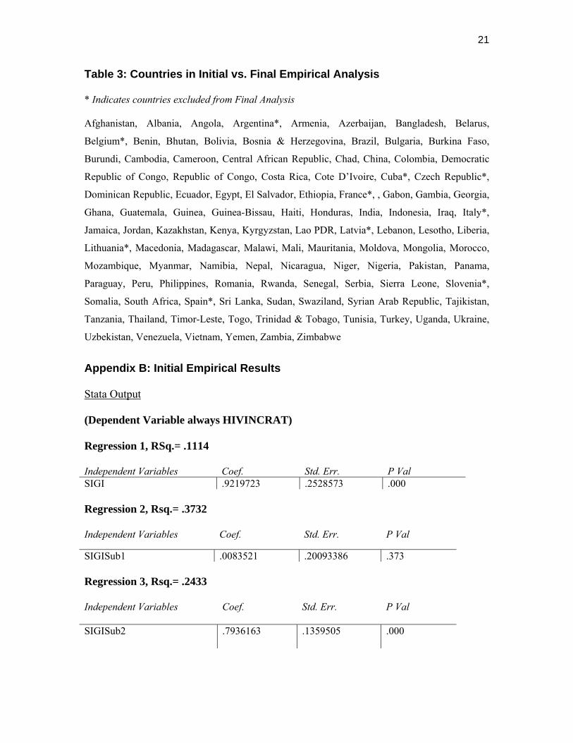
Appendix B: Initial Empirical Results

Stata Output

(Dependent Variable always HIVINCRAT)

Regression 1, RSq.= .1114 Independent Variables Coef. Std. Err. P Val SIGI .9219723 .2528573 .000 Regression 2, Rsq.= .3732 Independent Variables Coef. Std. Err. P Val

SIGISub1 .0083521 .20093386 .373 Regression 3, Rsq.= .2433 Independent Variables Coef. Std. Err. P Val

SIGISub2 .7936163 .1359505 .000

22

Regression 4, Rsq.= .0104 Independent Variables Coef. Std. Err. P Val

SIGISub3 -.1831828 .1737377 .294

Regression 5, Rsq.=.1490 Independent Variables Coef. Std. Err. P Val

SIGISub4 .5765528 .1338106 .000

Regression 6, Rsq.= 0.0334 Independent Variables Coef. Std. Err. P Val

SIGISub5 .2888175 .1509214 .058

Regression 7, Rsq.= .1873 Independent Variables Coef. Std. Err. P Val

Newindex .8255408 .1670219 .000

Regression 8, Rsq.= .3117 Independent Variables Coef. Std. Err. P Val

New Index .8300425 .2242562 .000

HIVprev 1.09E-07 4.75E-08 .024

GDPcap -.0000188 .0000161 .245

HealthExp .0001393 .0001644 .399

Muslim -.1537987 .0852894 .074

The above regressions provided valuable insight into which SIGI subindices are the most reliable indicators of female bargaining power. Additionally, they provide further evidence that variables such as Health Expenditure and Muslim Majority Dummy Variable do not belong in the final model. Interestingly, GDP/Capita did not generate a statistically significant result, yet GNI/Capita is statistically significant in the final model. These tables provide the evidence of a crucial step in arriving at the final product.

23

Abstract

Background: Currently, and in coming decades, populations in OECD countries are expected to age as fertility rates fall and life expectancies increase. It is anticipated that by 2050, nearly a quarter of the world’s population will be aged 60 or older. As a result of current demographic shifts and low interest rates in countries like Japan and in the Eurozone, orthodox monetary policies have become ineffective in stabilizing economies (culminating in the implementation of policies like quantitative easing). The effects of demographic transitions, such as population ageing, on the economy may therefore be more important than previously thought by economic researchers. Method: We hypothesize that interest rates are lower in ageing populations, due to changing attitudes towards savings and investments, which hence also generates a larger term spread. Three economic theories: the life-cycle hypothesis, the market segmentation theory, and the preferred habitat theory are used to analyze our empirical findings and interpretations. We explore the relationship between age and interest rates through the use of fixed effects (FE) and random effects (RE) estimation, and conduct several sets of regression analyses to test the robustness of the causal relationship between age and interest rates. Conclusion: We find that our results are consistent with our hypothesis: older populations generally have lower real short-term interest rates, and that the causal relationship is more statistically significant in relatively “old” countries compared to “young” countries. When economies are in a normal, non-recessionary state, our findings support our hypothesis that term spread is greater in ageing populations. During a recessionary period, our hypothesis that ageing populations have lower interest rates still holds, as we observe a smaller term spread (in the case of a convex yield curve) due to the effect of age.

Acknowledgments

First and foremost, we are grateful for being afforded the opportunity to write this thesis, as a requirement for our undergraduate degree in Global Economics (Honors Specialization). We wish to express our sincerest thank you to Professor Chris Robinson, our thesis supervisor, for providing us with valuable guidance and for supporting us throughout this research venture. We are also grateful to Professor Terry Sicular, Professor Tai-Yeong Chung, Professor Jacob Short, and Professor Alan Bester, from the Department of Economics at the University of Western Ontario, for their support and willingness to

24

help. We are extremely thankful for their sharing of expertise and knowledge, and are indebted to them. Last, but certainly not least, we take this opportunity to express gratitude to all of the department faculty members for their help and support, and especially to our peers who have directly, or indirectly, lent their hand in this venture. I. Introduction

Currently, and in coming decades, populations in OECD countries are expected to age as fertility rates fall and life expectancies increase. As the post-war “baby boom” generation moves through the demographic structure, it is anticipated that by 2050, nearly a quarter of the world’s population will be aged 60 or older, causing serious concerns for policy makers around the world (Bloom et al., 2011). The ramifications of demographic shifts on economic growth and stability are often overlooked in favour of more pertinent issues, like external factors related to foreign investments and trade. Due to current demographic shifts and low interest rates in countries like Japan and in the Eurozone, orthodox monetary policies have become ineffective in stabilizing economies (resulting in implementation of policies such as quantitative easing). As a result, the effects of demographic transitions on the economy may be more important than previously thought by economic researchers. Thus, for the purpose of our research paper, we aim to explore the effects of ageing on interest rates, in order to gain a greater perspective of the role of ageing populations on the economy. Our motivation for this topic stems from the recent implementation of Quantitative Easing (QE) as a monetary policy tool in several countries, including the United States, Japan, and the Eurozone. The main goal of monetary policy is to maintain economic stability with a low, stable inflation rate, and consistent output growth, which is usually achieved through the targeting of overnight interest rates. When interest rates are already very low, as is presently the case in many OECD countries, it is difficult to stimulate spending or achieve desired output levels in order to stabilize the economy, making interest rates as a tool for monetary policy virtually futile (OECD Statistics, 2015). Japan in particular, with the world’s oldest population, has long been suffering from what many economists call “a liquidity trap” (a phenomenon that renders monetary policies ineffective in stimulating consumption and investment through the targeting of lower interest rates, as interest rates are already very low or zero-bound). This has resulted in the employment of unconventional economic policies that have had various effects on its economy, such as excess reserves due to increased liquidity. Through the investigation of historical trends over the past few decades, we hypothesize that countries with older populations have lower interest rates as a consequence of changing savings and investment behaviours. In order to conduct our research, we collected panel data on a number of variables related to interest rates for 34 OECD nations, with the aim of using this data to empirically determine whether or not interest rates are, in fact, lower in older populations. We endeavour to explore the relationship between age and interest rates through the examination of (II) economic literature

25

pertaining to this topic, (III) our empirical model and econometric issues, (IV) our findings and analyses, and finally through (V) our general conclusions, which will summarize our findings regarding this research topic. II. Overview of Economic Literature and Background

It is widely acknowledged that many developed countries will experience ageing populations in the near future, posing several challenges for the economy. Much of the economic literature surrounding the topic of ageing populations concentrates on the general macroeconomic implications of demographic shifts, without specifically examining its effect on monetary policy tools, such as interest rates. Economic theories on savings and investment are unable to reach a definite conclusion as to how ageing populations will affect the economy, and in particular, whether this demographic transition will lower interest rates. While the effects of demographic shifts on ‘world interest rates’ have been explored in economic literature, there is not an abundance of information on the explicit effect of ageing populations on interest rates. Thus, for the purpose of contributing to economic research and thereby providing greater insight for future monetary policy implementation, we are motivated to determine whether or not a causal relationship exists between ageing and interest rates. (i) Determinants of Interest Rates

According to the IS-LM model developed by John Hicks in 1937, movements in investment and savings rates impact interest rates and concurrently, real GDP levels (Maes, 1989). Until the early 1990s, the majority of economic research on interest rates attempted to determine the factors that caused high interest rates around the world. An early paper written by Robert Barro and Xavier Sala-i-Martin (1990) investigates the reasons behind the high real interest rates across major industrialized countries in the 1980s, somewhat similar to our approach. Their paper discusses the importance of investment demand and desired savings in determining interest rates, and uses data from ten OECD nations to establish that high real interest rates yield positive shocks to investment demand and decrease desired savings. The authors identified favourable stock returns (which increased investment) and high oil prices as the “key elements” inducing high real interest rates in the early 1980s. By the early 2000s, the focus of economic research concerning interest rates shifted to determine why interest rates had declined to their lowest levels in decades. The majority of economic literature now concentrates on savings and investment changes as causes of the recent low real and nominal long-term interest rates. A paper by Ahrend et al. (2006) investigates the determinants of long-term interest rates in conventional economic models through the use of data from the United States. The authors find that three major factors including monetary policy credibility, saving-investment shifts, and portfolio shifts, account for the recent low real and nominal long-term bond yields. They postulate that yields on long-term bonds should show the expected path of future short-term interest rates. In particular, the study places emphasis on risk premia as the basis of the

26

‘expectations hypothesis’,1 and states that the real short-term interest rate (which reflects monetary policy actions) may be affected by changes in savings and investment, as well as portfolio shifts. In their conclusion, Ahrend et al. (2006) find that the main factor behind the changes in equilibrium real interest rates is the imbalance between savings and investment. The paper claims that the “underlying determinants” of these equilibrium real short-term interest rates include shocks to the marginal productivity of capital, the time preference (of long-term or short-term investments), expected future income, and demographic shifts. Furthermore, a paper published in 2005 by the IMF (2005) explores savings and investment from a global perspective. It suggests that a “global savings glut” is responsible for causing an excessive amount of savings and hence the decline of interest rates during that period. Additionally, it blames the 1997 Asian Financial Crisis for lower investment levels in the early 2000s, and indicates that in an increasingly global economy, the significant change in the early 2000s from a deficit to a surplus in savings was the main cause of low long-term real interest rates around the world. The distribution of savings and investment also has considerable effects on a country’s current account balance, particularly in the United States where the deficit in 2005 reached record levels (Bernanke, 2005). This shift in the current account balance, however, was not the only driver of low real interest rates in that year. The savings-investment imbalance was further spurred by key factors such as demographic shifts, declines in public savings, and financial sector reforms (IMF, 2005). All in all, it is clear from economic literature that opinions vary on the determinants of interest rates, which are made even more complicated by the global interactions of open economies. From a changing demographics perspective, we must look at how ageing populations will impact the determinants of interest rates. Therefore, for the purposes of our research paper, we will focus on the impact of ageing on interest rates through savings and investment, as the majority of economic literature agrees that these two factors are influenced heavily by demographic factors such as age.

(ii) Savings and the Life-Cycle Hypothesis

The majority of research surrounding ageing and savings is explained by the life-cycle hypothesis, a theory first proposed by Modigliani and Brumberg (1954). The life-cycle hypothesis suggests that households want to smooth consumption over their lifetime given their income, implying that savings rates increase with income during an individual’s working life, and then decline (and eventually becomes negative) during retirement (Bosworth et al., 2004). In accordance with this theory, countries with a longer life expectancy will generally have higher private savings rates, as more people approach the retirement age. This, in

1The hypothesis that long-term rate is the sum of expected short-term rates plus a term premium, in both the present and future and that the shape of the yield curve depends on these market expectations (Wheelock et al., 2009).

27

turn, theoretically prompts central monetary authorities to suppress interest rates in order to stimulate consumption and investment (as the IS-LM model shows that interest rates adjust to equate saving and investment). As the process of ageing continues, private savings rates will start to decline, as households draw into their savings after retirement. Public savings may also shrink as more pressure is put on governments to spend on public pensions and medical care in order to support ageing populations. (iii) Investment, the Preferred Habitat Theory, and the Market Segmentation

Theory   According to conventional term structure models, shifts in portfolio preferences can affect bond yields through changes in term premia and risk premia (Ahrend et al. 2006). These changes could be a result of shifting perceptions, attitudes of investors towards risk, or perhaps the redistribution of wealth. Increases in the demand for long-term government bonds relative to supply, or movements towards investors that are less risk averse, will act to decrease premia and compress yields, even when there are no changes in expected inflation or equilibrium real interest rates (Ahrend et al. 2006). As such, it follows that with respect to ageing populations, older investors prefer short-term investments that are less risky, which should act to decrease premia and yields in the short term and increase them in the long term, giving us a larger term spread (steeper yield curve). This hypothesis is supported by an extension of the expectations theory called the “preferred habitat theory”. There are several interpretations of the expectations theory, but all suggest that forward rates are equivalent to expected spot rates (Cox et. al, 2007). In other words, it suggests that long-term interest rates can predict future short-term interest rates, and thus predict the yield curve. The preferred habitat theory extends this hypothesis and explains why bond yields are higher in the long term than in the short term. It suggests that in addition to expectations of return, potential investors also have a preferred maturity length for the bonds they choose to invest in, called their “preferred habitat”. Therefore, in order to incentivize people to invest outside of their preferred habitat (maturity length), they must be compensated with higher returns (higher interest rates). In addition to the preferred habitat theory of term structure, we also look at the market segmentation theory. The market segmentation theory suggests that long-term and short-term interest rates are not related and move independently of each other, and that the yield curve is shaped according to the supply and demand for bonds with different maturity dates. Given that older investors have to be compensated for the higher risks associated with holding assets for a longer period, especially since they prefer more liquid assets, this theoretically lowers bond prices and drives up interest rates in the long term (preferred habitat theory) (Murphy et al., 2000). Thus, in accordance with these two theories, we hypothesize that the term spread will be greater (a steeper yield curve) in an ageing population.

28

Cooper and Kaplanis (2000), however, find evidence that international capital markets are neither fully integrated nor segmented. This contradicts the market segmentation theory in that the movement of long-term and short-term interest rates are not totally independent of each other in reality. In their paper, the authors identify studies by Errunza and Losq (1985), Jorion and Schwartz (1986), Cooper and Kaplanis (1986, 1994), Hietala (1989), French and Poterba (1991) and Tessar and Werner (1995), which provide empirical evidence that models of fully integrated or segmented international capital markets are unable to explain trends in portfolio shifts or the behaviour of security returns completely, implying that markets are perhaps not as segmented as the theory suggests. With decreasing fertility rates and higher life expectancies, it seems that traditional economic policies, especially monetary policies, will no longer work effectively. Increased old dependency ratios will negatively impact GDP levels and GDP per capita growth rates, widening the output gap, and lowering productivity levels. A slowdown in population growth and higher life expectancies also imply lower labour force growth rates, as the number of people entering the workforce is not enough to offset the number of people leaving. As a result, less investment is needed to maintain capital stock, subsequently decreasing investment demand and lowering interest rates in the economy (Turner et al. 1998). These mechanisms suggest that under such circumstances, ageing populations will lower interest rates, rendering orthodox monetary policy useless. III. Our Model

In order to assess the impact of ageing populations on world interest rates, we collected panel data from all 34 OECD member countries, and ran various regressions to evaluate the robustness of the relationship between the age of a population and interest rates. We chose to focus on OECD countries as they account for approximately 51 percent of the total world GDP (PPP measure, OECD Statistics, 2010), and are all classified as developed countries by the United Nations. Our variables of interest are represented by three different measures of age in our empirical model: median age (medage), the old dependency ratio (dependencyratio) and the percentage of the population above 65 (pcpop65). We chose to use median age as our primary method of age measurement as this is a common practice across economic literature, and continues to be the most widely used measure in population ageing. However, in order to affirm the strength of our hypothesis, we also chose two other common population age indicators. The old dependency ratio is measured by dividing the number of people over 65 by the number of people in the working age population. The higher the ratio, the more people in retirement that are financially “depending” on a worker. Finally, we use the percentage of the population over 65 as a population age indicator, as this allows us to account for the specific segment of the population that is made up of people in their retirement age. Additionally, two separate measures of interest rates were used for our dependent variable in order to get a more holistic overview of the causal relationship between age and interest rates: real short-term interest rates (rstir) and the term spread (termspread).

29

Short-term interest rates are the tools used by central banks to implement monetary policies. They represent either the three-month interbank offer rate, or securities of three-month maturities (such as Treasury bills), which are used to affect any economic changes in the immediate run (OECD Statistics, 2015). The term spread, which is calculated by the long-term interest rate (10-year maturity bonds) less the short-term interest rate (3-month maturity bonds), is equivalent to the slope of the yield curve (Aksoy, Basso, 2014). We therefore ran the following regressions on our three measures of age (denoted as ‘agemeasure’):

0 1 2 3 4

5 6 7 8

9 10 11 _ _

it it it it

it it it it

itit it it

rstir a a agemeasure a grosssave a exrate a lforcegrow

a grosscapform a govtdebt a stockspcgdp a fdi

a infl a riskpre a curr acc bal e

0 1 2 3

4 5 6

7 8 9 10

11 _ _

it it it

it it it

it it it it

itit

termspread b b agemeasure b grosssave b exrate

b lforcegrow b grosscapform b govtdebt

b stockspcgdp b fdi b infl b riskpre

b curr acc bal u

Note: i denotes country and t denotes year. In our regression analyses, we included inflation rates (infl), exchange rates (exrate), gross savings rates (grosssave), gross capital formation (grosscapform), labour force growth rates (lforcegrow), the risk premium on lending (riskpre), the total value of stocks traded as a share of GDP (stockspcgdp), foreign direct investments (fdi), government debt (govtdebt), and the current account balance (curr_acc_bal) as control variables, since they play a major role in determining interest rates. Inflation rates were included as they are good indicators of the central banks’ monetary policy actions, and because interest rates are adjusted according to inflation rate targets. Gross savings rates and gross capital formation act to reflect domestic consumer and investors’ confidence, which in turn affect inflation and interest rates. The value of stocks traded as a percentage of GDP, the risk premium on lending and foreign direct investments are good measures of international investment decisions, while exchange rates, and the current account balance are indicators for foreign trade, international currency positions and subsequently, the balance of payments (BoP) accounts of countries (Hodgson et al., 1998). Furthermore, labour force growth is an important determinant of interest rates as explained earlier, and can be negatively impacted by an ageing population. An older population implies lower labour force growth rates, which could decrease the capital stock in the economy when the labour market shrinks. According to Ahrend et al. (2006), productivity, output and investment levels are consequently affected, and fluctuations in interest rates follow. Lastly, government debt was included in our empirical model

30

because studies show that increasing government debt negatively impacts the value of household assets, in turn affecting interest rates through altered consumption and investment levels (Engen, Hubbard, 2004).

Figure A: An illustration of the effect of ageing on the term spread [ab > xy], as explained by the Preferred Habitat Theory and the Market Segmentation Theory

As explained by the life-cycle hypothesis, we expect to see a negative correlation between real short-term interest rates and our age measures. Moreover, with support from the preferred habitat theory and the market segmentation theory, we expect to see a larger term spread (steeper yield curve) in ageing populations. This is illustrated in Figure A above, where ab > xy when the elderly demand more short-term bonds, and when the movement of long-term and short-term interest rates are independent of each other (Occhino, 2008). IV. Econometric Considerations (i) Endogeneity

The control variables added in our regression analyses are the main determinants of interest rates, reflecting mainly domestic consumer and investor confidence, savings and investment behaviour, the central bank’s monetary policy actions, as well as external factors such as international trade and investments. However, due to the complexities of world financial and capital markets, the existence of some non-quantifiable factors like market expectations, as well as our inability to collect qualitative data such as the elderly’s expectations of changing pension plan schemes in each OECD country, the problem of omitted variable bias is virtually inevitable (Akerlof, 2002). Moreover, given the macroeconomic nature of our research project, the issue of reverse causation is likely to be present since many macroeconomic indicators are determined simultaneously. For example, it might be the case that higher gross savings (and lower

31

consumption expenditure) result in lower interest rates in a bid to stimulate the economy. Concurrently, higher interest rates could cause consumption levels to fall due to the higher costs of borrowing, and hence culminate in higher gross savings rates. Thus, our econometric model is likely to be subject to simultaneity bias, and we recognize the need to use alternative methods of estimation other than pooled OLS, as the Gauss-Markov assumption of exogeneity is violated (Nakamura and Nakamura, 1998). It is also likely that our model suffers from measurement error due to inconsistent data collection methods, and incorrect statistical reporting across 34 OECD countries. This could make our findings on age measures inaccurate measures of the causal effect between age and our two dependent interest rate variables. Therefore, we acknowledge that our model is not perfect in capturing the true effect between age and interest rates, and our coefficient of determination (R2) values of 0.3 to 0.5 across our general 1970-2013 regressions may also suggest that there are more factors affecting interest rates that we have not included in our empirical model. (ii) Heteroskedasticity

The problem of heteroskedasticity is prevalent in time-series panel data analysis due to autocorrelation (variation within each country across time), temporal correlation (variation across countries in one period of time) and the inertia of persistent common shocks (Reimers and Harvey, 2011). As a result of different economic policies across OECD member countries, it is not surprising to see cross-country variation among our independent variables. According to Reimers and Harvey (2011), within-country variation is also inevitable, as individuals differ, for example, in income levels and preferences. We therefore use White standard errors to reduce biases in our test statistics and confidence intervals arising from heteroskedasticity. Given the susceptibility of our model to the various econometric issues mentioned above, OLS estimation is unlikely to give us unbiased or efficient results (Nakamura and Nakamura, 1998). Thus, we estimate our model using both random effects (RE) and fixed effects (FE) estimation; a common method used across economic literature for panel data. The employment of FE estimation allows us to remove any unobserved time-constant variables that may be correlated with our explanatory variables. We assume strict exogeneity, and hence the FE method of estimation proves to be a powerful tool in removing omitted variable bias and abating the problem of endogeneity. However, we cannot ensure that our variables of interest, particularly median age, have enough variability over time for FE to produce the most accurate results. As such, we compare each set of our FE results with RE estimation. While RE is the less robust measure, it allows us to estimate the effects of time-invariant factors and gives smaller standard errors. However, it is important to note that RE estimated coefficients may be biased, as they do not account for omitted variable bias. Therefore, in order to mitigate these econometric issues and gain a holistic understanding of the relationship between age and interest rates, we estimate our model using both FE and RE strategies.

32

V. Empirical Evidence and Analysis

In order to reduce biases in our regression coefficients resulting from the large amounts of missing data in the 1970s and 1980s, we ran regressions for two different time subsets: 1970-2013 and 1990-2013. The results from RE and FE estimation differ slightly due to reasons mentioned in section (III), but ultimately support our hypothesis. As the two time subsets produce similar results for both methods of estimation especially for real short-term interest rates, we will continue to test our hypothesis with the full data set ranging from 1970-2013, as it accounts for a wider time frame and contains more data. In general, we find the FE coefficients of our three measures of age to be significant at a 5 percent level and negatively correlated with real short-term interest rates, supporting our hypothesis (see Table 1). However, we observe a weaker statistical significance, ranging from 10 percent to 20 percent, for the coefficients of our age measures in our term spread regressions, perhaps suggesting that age is less likely to affect the term spread to a large extent, in comparison to real short-term interest rates. We nonetheless find a positive correlation between our age measures and the term spread, which runs in tandem with our hypothesis. Thus, our results are encouraging overall, because the negative (positive) correlation between our age measures and the real short-term interest rate (the term spread) concurs with our hypothesis that ageing populations have lower interest rates. In the following sub-sections, we will use the life-cycle hypothesis, the market segmentation theory, and the preferred habitat theory to analyze our findings, to ultimately determine the robustness of the causal relationship between age and interest rates. (i) Comparison of Age Effects in Young and Old Countries

In order to test the robustness of the relationship between age and interest rates, we ran two separate sets of regressions of our dependent variables (real short-term interest rates and the term spread) on our age measures, for a group of relatively “young” and “old” countries in terms of average median age. Our “young” countries consist of Turkey, Mexico, Israel and Chile, while our “older” countries include Japan, Germany, Canada and Finland. Through this, we observe that while all three of our age measures are negatively correlated with real short-term interest rates, the relationship is more statistically significant in older countries (at a 1 percent level) compared to younger countries, in which median age is the only statistically significant age measure (at a 5 percent level) (see Table 2). In countries with the lowest average median age, the coefficients for the old dependency ratio and percentage population over 65 are not significant at a plausible level. Alluding to the life-cycle hypothesis, savings rates increase (and consumption expenditure decreases) as a population ages, because individuals near the end of their working lives start saving intensively for their retirement (Ahrend et al. 2006). This subsequently puts a downward pressure on inflation rates, which in turn, prompts central

33

Table 1: All Countries General Regressions

Table 2: Countries with High and Low Average Median Age

1970‐2013 1990‐2013MedianAge

(RE) (FE) (RE) (FE)Real

InterestRate

‐0.223(0.066)

z:‐3.36P>|z|:0.001

***

‐0.638     (0.272)

t: ‐2.34         P>|t|: 0.029 

**

‐0.223 (0.066)

z:‐3.36P>|z|:0.001

***

‐0.638     (0.272)

t: ‐2.34         P>|t|: 0.029 

**

TermSpread

0.097(0.001)

z:2.10P>|z|:0.035

**

0.160     (0.093)

t: 1.73        P>|t|: 0.098 

*

0.090(0.049)

z:2.10P>|z|:0.035

**

0.099     (0.071)

t: 1.39       P>|t|: 0.180

DependencyRatio (RE) (FE) (RE) (FE)

RealInterestRate

‐0.050(0.046)

z:‐1.09P>|z|:0.278

 ‐0.558    (0.234) 

t: ‐2.38         P>|t|: 0.027 

**

‐0.050 (0.046)

z:‐1.09P>|z|:0.278

‐0.558 (0.234)

t: ‐2.38         P>|t|: 0.027 

**TermSpread

0.023(0.044)

z:0.51P>|z|:0.609

0.120    (0.092)

t: 1.30        P>|t|: 0.206

0.022 (0.044)

z:0.50P>|z|:0.620

0.069 (0.107)

t: 0.64         P>|t|: 0.528

PercentagePopulationOver65

(RE) (FE) (RE) (FE)Real

InterestRate

‐0.151(0.061)

z:‐2.45P>|z|:0.014

**

‐1.298     (0.371)

t: ‐3.50     P>|t|: 0.002 

***

‐0.151 (0.061)

z:‐2.45P>|z|:0.014

**

‐1.298     (0.371)

t: ‐3.50  P>|t|: 0.002 

***

TermSpread

0.098(0.057)

z:1.72P>|z|:0.085

*

0.218     (0.145)

t: 1.51       P>|t|: 0.146

0.097 (0.057)

z:1.72P>|z|:0.086

*

0.206 (0.161)

t: 1.28       P>|t|: 0.216

HighestAverageMedianAge LowestAverageMedianAgeMedianAge

(RE) (FE) (RE) (FE)

RealInterestRate

‐0.515(0.131)

z:‐3.93P>|z|:0.000

***

‐0.524 (0.024)

t:‐21.51P>|t|:0.000

***

‐1.269 (0.566)

z:‐2.24P>|z|:0.025

**

‐1.168(0.236)

t:‐6.90P>|t|:0.006

***

TermSpread

0.034(0.065)

z:‐0.52P>|z|:0.602

‐0.048(0.041)

t:‐1.16P>|t|:0.331

0.537(0.466)

z:1.15P>|z|:0.249

‐0.390(0.484)

t:0.81P>|t|:0.479

DependencyRatio (RE) (FE) (RE) (FE)

RealInterestRate

‐1.269(0.002)

z:‐3.09P>|z|:0.002

***

‐0.404 (0.216)

t:‐18.78P>|t|:0.000

***

‐0.878 (0.768)

z:‐1.15P>|z|:0.248

‐1.592(0.839)

t:‐1.90P>|t|:0.154

TermSpread

‐0.040(0.028)

z:‐1.44P>|z|:0.149

‐0.101 (0.037)

t:‐2.75P>|t|:0.070

*

‐0.375 (0.527)

z:0.71P>|z|:0.477

‐0.015(0.912)

t:‐0.02P>|t|:0.388

PercentagePopulationOver65

(RE) (FE) (RE) (FE)Real

InterestRate

‐0.487(0.139)

z:‐3.50P>|z|:0.000

***

‐0.656 (0.049)

t:‐13.53P>|t|:0.001

***

‐1.462 (0.831)

z:‐1.76P>|z|:0.079

*

‐3.403(2.381)

t:‐1.43P>|t|:0.248

TermSpread

‐0.060(0.055)

z:‐1.10P>|z|:0.273

‐0.135 (0.052)

t:‐2.61P>|t|:0.080

*

‐0.321 (0.279)

z:‐1.15P>|z|:0.249

‐2.091(1.153)

t:1.81P>|t|:0.167

34

banks to lower short-term nominal interest rates1, in order to stimulate consumption and investment. We find the coefficients of all three age variables to be more significant in countries with a higher average median age than in those with a lower average median age, indicating that age may play a larger role in affecting interest rates in older populations. The life-cycle hypothesis provides an explanation for this phenomenon, as people tend to save more as they get older and approach their retirement age. With reference to our regressions of the term spread, we generally find statistically insignificant results for all three of our age measures. Moreover, the observation of a negative correlation between the age variable (pcpop65) and the term spread, is not consistent with our hypothesis, or the preferred habitat and market segmentation theories. Therefore, it is likely that in reality, markets are not as segmented as economic theory states, providing explanations for the negative instead of positive correlation that we expected to find, as well as less significant results. (ii) Comparison of Age Effects in ‘Slowly’ and ‘Rapidly’ Ageing Populations

In order to further explore the relationship between age and interest rates, we also compare countries that have aged the most rapidly in terms of median age, and those that have aged the most slowly in terms of median age, over the years 1970-2013. We find highly statistically significant results (at a 1 percent level) for all measures of age with real interest rates in the subset of rapidly ageing countries (see table 3). This implies that in countries with populations that have aged most rapidly in terms of median age, population age has a larger impact on interest rates, than in their slowly ageing counterparts. The coefficients are all negatively correlated with real short-term interest rates, which are once again, consistent with our hypothesis and supported by the life-cycle theory (see table 3). With regards to the term spread, we see some mixed results in terms of the correlation with our age measures. We observe that in rapidly ageing countries, age is negatively correlated with term spread, whereas in slowly ageing countries, it is positively correlated, though not statistically significant for our FE regressions (see table 3). We expected to see a larger term spread in more rapidly ageing countries, as we observed a statistically significant negative correlation with interest rates and our three age measures. Nevertheless, our hypothesis may still be supported by these findings if the movement of short-term and long-term interest rates is interdependent, as this would generate a yield curve with a smaller slope. In other words, these results may suggest that the market segmentation theory may not hold true, although more research beyond the scope of this paper would be needed in order to determine the term structure.

1 The Fisher equation: r = i – π demonstrates the linear relationship between real and nominal interest rates, where i represents the nominal interest rate, r represents the real interest rate, and π represents inflation.

35

Table 3: Countries with Rapid and Slow Changing Age Distributions

(iii) Changing Age Distributions of “Young” Countries

Given that we have found a causal relationship between age and interest rates in rapid and slow ageing populations, we decided to test this relationship in countries that were relatively the same in terms of median age in 1970 - that is to say, countries with the same approximate starting point. We identify two different subsets of countries that were “young” in 1970, with one group ageing faster than the other. Our “young and rapidly ageing” countries consisted of Canada, Chile, and Ireland, while our “young and slowly ageing” subset included Israel, Portugal, and Slovak Republic. Overall, we find fairly different results between the two estimation methods in this robustness check, compared to our previous estimations. While this may have some interesting implications for our hypothesis, it is important to note that this may also be a result of a smaller data set, and the fact that it was difficult to ensure countries had approximately the same median age in 1970. With real short-term interest rates, we find highly statistically significant results at the 1 percent level for all three age measures when using RE estimation within the countries that have had the fastest changing age distributions (see table 4). This is not the case for our RE estimates in slowly ageing countries, as only the variable accounting for the population over 65 is statistically significant. In both subsets, our findings reveal that the

RapidAgeing SlowAgeingMedianAge

(RE) (FE) (RE) (FE)Real

InterestRate

‐0.394    (0.084)

z: ‐4.69     P>|z|: 0.000 

***

‐0.358    (0.036)

t: ‐9.95     P>|t|: 0.002 

***

‐1.457     (0.271)

z: ‐5.37     P>|z|: 0.000 

***

‐1.325    (0.264)

t: ‐5.02     P>|t|: 0.015 

**

TermSpread

‐0.114    (0.049)

z: ‐2.36      P>|z|: 0.018 

**

‐0.137    (0.067)

t: ‐2.03      P>|t|: 0.135

‐0.433     (0.074)

z: 5.90      P>|z|: 0.000 

***

0.324     (0.523)

t: 0.62      P>|t|: 0.580

DependencyRatio (RE) (FE) (RE) (FE)

RealInterestRate

‐0.185    (0.055)

z: ‐3.35      P>|z|: 0.001 

***

‐0.323    (0.062)

t: ‐5.17      P>|t|: 0.014 

**

‐0.118    (0.283)

z: 0.420      P>|z|: 0.677

‐0.917    (0.269)

t: ‐3.40      P>|t|: 0.043 

**

TermSpread

‐0.076    (0.013)

z: ‐5.96     P>|z|: 0.000 

***

‐0.162    (0.078)

t: ‐2.08     P>|t|: 0.130

‐0.043    (0.058)

z: 0.76     P>|z|: 0.448

0.486     (0.434)

t: 1012     P>|t|: 0.345

PercentagePopulationOver65 (RE) (FE) (RE) (FE)

RealInterestRate

‐0.351    (0.106)

z: ‐3.32    P>|z|: 0.001 

***

‐0.605    (0.082)

t: ‐7.42    P>|t|: 0.005 

***

‐0.609   (0.538)

z: ‐1.12    P>|z|: 0.261

‐1.482    (0.186)

t: ‐7.95    P>|t|: 0.004 

***

TermSpread

‐0.123    (0.029)

z: ‐4.31      P>|z|: 0.000 

***

‐0.256    (0.118)

t: ‐2.17      P>|t|: 0.119 

‐0.344    (0.116)

z: 2.96      P>|z|: 0.003 

***

0.648     (0.342)

t: 1.90      P>|t|: 0.154

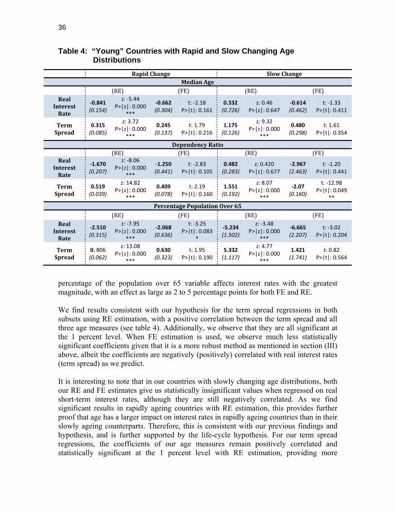
36

Table 4: “Young” Countries with Rapid and Slow Changing Age Distributions

percentage of the population over 65 variable affects interest rates with the greatest magnitude, with an effect as large as 2 to 5 percentage points for both FE and RE. We find results consistent with our hypothesis for the term spread regressions in both subsets using RE estimation, with a positive correlation between the term spread and all three age measures (see table 4). Additionally, we observe that they are all significant at the 1 percent level. When FE estimation is used, we observe much less statistically significant coefficients given that it is a more robust method as mentioned in section (III) above, albeit the coefficients are negatively (positively) correlated with real interest rates (term spread) as we predict. It is interesting to note that in our countries with slowly changing age distributions, both our RE and FE estimates give us statistically insignificant values when regressed on real short-term interest rates, although they are still negatively correlated. As we find significant results in rapidly ageing countries with RE estimation, this provides further proof that age has a larger impact on interest rates in rapidly ageing countries than in their slowly ageing counterparts. Therefore, this is consistent with our previous findings and hypothesis, and is further supported by the life-cycle hypothesis. For our term spread regressions, the coefficients of our age measures remain positively correlated and statistically significant at the 1 percent level with RE estimation, providing more

RapidChange SlowChangeMedianAge

(RE) (FE) (RE) (FE)Real

InterestRate

‐0.841    (0.154)

z: ‐5.44     P>|z|: 0.000 

***

‐0.662    (0.304)

t: ‐2.18     P>|t|: 0.161

0.332     (0.726)

z: 0.46     P>|z|: 0.647

‐0.614    (0.462)

t: ‐1.33     P>|t|: 0.411

TermSpread

0.315     (0.085)

z: 3.72      P>|z|: 0.000 

***

0.245     (0.137)

t: 1.79      P>|t|: 0.216

1.175     (0.126)

z: 9.32      P>|z|: 0.000 

***

0.480     (0.298)

t: 1.61      P>|t|: 0.354

DependencyRatio (RE) (FE) (RE) (FE)

RealInterestRate

‐1.670    (0.207)

z: ‐8.06      P>|z|: 0.000 

***

‐1.250    (0.441)

t: ‐2.83      P>|t|: 0.105

0.482     (0.283)

z: 0.420      P>|z|: 0.677

‐2.967    (2.463)

t: ‐1.20      P>|t|: 0.441

TermSpread

0.519    (0.039)

z: 14.82     P>|z|: 0.000 

***

0.409    (0.078)

t: 2.19     P>|t|: 0.160

1.551     (0.192)

z: 8.07     P>|z|: 0.000 

***

‐2.07     (0.160)

t: ‐12.98    P>|t|: 0.049 

**PercentagePopulationOver65

(RE) (FE) (RE) (FE)Real

InterestRate

‐2.510    (0.315)

z: ‐7.95    P>|z|: 0.000 

***

‐2.068    (0.636)

t: ‐3.25    P>|t|: 0.083 

*

‐5.234   (1.502)

z: ‐3.48    P>|z|: 0.000 

***

‐6.665    (2.207)

t: ‐3.02    P>|t|: 0.204

TermSpread

0. 806    (0.062)

z: 13.08      P>|z|: 0.000 

***

0.630     (0.323)

t: 1.95      P>|t|: 0.190

5.332     (1.117)

z: 4.77      P>|z|: 0.000 

***

1.421     (1.741)

t: 0.82      P>|t|: 0.564

37

evidence in support of our hypothesis, the market segmentation theory, and the preferred habitat theory (see table 4). To reiterate, the results from our analyses above suggest that population age plays a bigger role in determining interest rates in rapidly ageing populations as opposed to slowly ageing populations, regardless of their initial median age in 1970. Policymakers in rapidly ageing countries may thus need to be more cognizant of their ageing populations when making monetary policy decisions, as these results indicate that traditional monetary policy may not work as well. (iv) Recessionary Period Analysis

So far, our analyses of the effect of ageing on interest rates assume that economies operate in a normal state (a non-recessionary period). In order to test our hypothesis as well as the robustness of the effect of ageing on interest rates further, we examine the relationship between these two variables during a recession1. In particular, we will focus on the 2008 U.S Financial Crisis due to the rippling economic effects it had on global markets and OECD nations, as well as the 2010 European Union (EU) Debt Crisis, since 21 out of the 34 member countries of the OECD are members of the EU (OECD Statistics, 2015). With reference to Figure B, which shows a convex yield curve in a recession, we hypothesize that the term spread will be smaller, i.e. |xy| < |ab| (Ang et al, 2006). In accordance with the preferred habitat theory, older investors must be compensated with higher returns if they hold bonds for a longer term, or a term outside of their “preferred habitat”. Subsequently, a greater demand for bonds of a shorter term, by the elderly, will act to lower short-term yields (Cox et. al, 2007). In addition, assuming that the market segmentation theory holds, long-term interest rates do not influence short-term interest rates. Thus, we predict that these combined effects will pull the convex yield curve lower, as can be seen in Figure B, consequently generating a smaller term spread during a recessionary period. The following sub sections: (a) 2008 Financial Crisis, and (b) 2010 EU Debt Crisis summarize our findings in seeking to test the robustness of the causal relationship between age and interest rates. (a) 2008 Financial Crisis

With the aim of examining if the term spread is indeed smaller during a recession as a result of age, we interacted all three of our age measures with a 2008 time dummy, representing the initial onset of the financial crisis. We then compared them with our regular estimates from the same regression, representing a stable economic period. Our results were encouraging as they were consistent with our prediction: a recessionary period will yield a smaller term spread (negative correlation between the term spread and age measures).

1 A recession is typically defined as two consecutive quarters of negative GDP growth in an economy.

38

Figure B: An illustration of the effect of ageing on the term spread |xy| <

|ab| during a recession, as explained by the Preferred Habitat Theory and the Market Segmentation Theory

We therefore ran the following regressions:

0 1 2 3

4 5 6 7

8 9 10 11

12

* 2008

_ _

it it it

it it it it

it it it it

itit

rstir c c agemeasure c agemeasure d c grosssave

c exrate c lforcegrow c grosscapform c govtdebt

c stockspcgdp c fdi c infl c riskpre

c curr acc bal e

0 1 2 3

4 5 6

7 8 9 10

11 12

* 2008

_ _

it it it

it it it

it it it it

itit it

termspread g g agemeasure g agemeasure d g grosssave

g exrate g lforcegrow g grosscapform

g govtdebt g stockspcgdp g fdi g infl

g riskpre g curr acc bal u

Note: where i denotes country and t denotes year.

Referring to Table 5, both our FE and RE estimates of the interacted terms (age measures and the 2008 year dummy) with the term spread are negatively correlated, signalling a smaller term spread during a recessionary period. However, none of the estimates of our interacted terms were significant at a 5 percent level, perhaps indicating that age was less likely to affect term spread. Interestingly, we also observe the magnitude of the interacted

39

terms to be relatively larger than our regular age estimates, demonstrating that the effect of age on interest rates, and term spread specifically, is larger during a recession as opposed to a more stable economic period.

Table 5: 2008 Financial Crisis

Given that asset liquidity tends to decline during a recession due to tighter market conditions and credit constraints, older investors start buying safer, short-term assets that have greater liquidity (Gibson and Mougeot, 2004). In turn, this requires them to tap into their personal savings, which will ultimately act to affect interest rates, in accordance with the life-cycle hypothesis. Therefore, this mechanism seems to suggest that age should have a larger impact on the term spread during a recession, as savings and investment rates (both of which are highly influenced by an ageing population) move to influence interest rates. For our regressions of the real short-term interest rate on our age measures, we also find results that support our hypothesis: lower interest rates in older populations. Table 5 shows that both our FE and RE estimates of all interacted terms (age measures and time dummies) are negatively correlated with the real short term interest rate, indicating that interest rates are indeed lower in ageing populations. Overall, our RE and FE estimates have strong statistical significance levels of 1 percent and 5 percent respectively, and we also notice larger coefficients of our interacted age variables with the real short-term interest rate, as compared to the non-interacted terms (see table 5). This could be due to the fact that governments commonly buy more short-term bonds during the initial hit of a financial crisis, in a bid to lower interest rates (Gibson and Mougeot, 2004). Thus, this

MedianAge

medage*d2008

(RE)medage*d2008

(FE)medage(RE)

medage(FE)

RealInterestRate

‐1.320(0.507)

z:‐2.60p>|z|:0.009

***

‐1.232(0.513)

t:‐2.40p>|t|:0.026

**

‐0.170(0.051)

z:‐3.33p>|z|:0.001

***

‐0.593(0.276)

t:‐2.15p>|t|:0.043

**TermSpread

‐0.142(0.337)

z:‐0.42p>|z|:0.673

‐0.129(0.425)

t:‐0.30p>|t|:0.765

0.044(0.042)

z:1.05p>|z|:0.296

0.073(0.063)

t:1.15p>|t|:0.261

PercentagePopulationOver65

pcpop65*d2008

(RE)pcpop65*d2008

(FE)pcpop65(RE)

pcpop65(FE)

RealInterestRate

‐1.524(0.432)

z:‐3.52p>|z|:0.000

***

‐1.220(0.518)

t:‐2.36p>|t|:0.028

**

‐0.127(0.046)

z:‐2.76p>|z|:0.006

***

‐1.197(0.368)

t:‐3.26p>|t|:0.004

***

TermSpread

‐0.133(0.315)

z:‐0.42p>|z|:0.671

‐0.125(0.439)

t:‐0.290p>|t|:0.778

0.093(0.371)

z:2.50p>|z|:0.012

**

0.148(0.165)

t:0.900p>|t|:0.380

DependencyRatio

dependencyratio*

d2008(RE)dependencyratio*

d2008(FE)dependencyratio

(RE)dependencyratio

(FE)Real

InterestRate

‐1.426(0.425)

z:‐3.35p>|z|:0.001

***

‐1.267(0.580)

t:‐2.190p>|t|:0.040

**

‐0.400(0.042)

z:‐0.96p>|Z|:0.337

‐0.485(0.231)

t:‐2.10p>|t|:0.048

**TermSpread

‐0.121(0.344)

z:‐0.35p>|Z|:0.725

‐0.126(0.451)

t:‐0.280p>|t|:0.782

0.016(0.054)

z:0.29p>|Z|:0.773

0.040(0.200)

t:0.360p>|t|:0.720

40

effect, compounded with the greater demand of short-term bonds by the elderly, provides an explanation for why we see a larger negative impact of age on interest rates during the 2008 Financial Crisis. (b) 2010 EU Debt Crisis

The 2010 EU Debt Crisis had severe economic ramifications on EU member

countries, given the high volume of trading and investment activity within the European Economic Union (Brenton and Manchin, 2003). Therefore, in order to test the effect of ageing on interest rates during this period of economic downturn in the region, we tested our regression model on EU member countries within the OECD. We interacted our age measures with a 2010 time dummy to properly examine the relationship between these two factors during a recession, and subsequently compared it to our regular estimates, as we did above for our analysis on the 2008 Financial Crisis. In general, we find results that are consistent with our prediction using both RE and FE estimation methods: a negative correlation between our interacted age measures, and both the term spread, and the real short-term interest rates. Moreover, our estimates of all three interacted age terms on the term spread are statistically significant at a 5 percent level for both methods of estimation (see table 6). We ran the following regressions:

0 1 2 3

4 5 6

7 8 9 10

11 12

* 2010

_ _

it it it

it it it

it it it it

itit it

rstir h h agemeasure h agemeasure d h grosssave

h exrate h lforcegrow h grosscapform

h govtdebt h stockspcgdp h fdi h infl

h riskpre h curr acc bal e

0 1 2 3

4 5 6

7 8 9 10

11 12

* 2010

_ _

it it it

it it it

it it it it

itit it

termspread j j agemeasure j agemeasure d j grosssave

j exrate j lforcegrow j grosscapform

j stockspcgdp j fdi j infl j riskpre

j riskpre j curr acc bal u

Note: where i denotes country and t denotes year.

Interestingly, in this set of analysis, we find that our FE coefficients of the interacted age terms, which account for the 2010 EU Debt Crisis, are about six times larger than the regular age measures. This could possibly be due to the implementation of unconventional monetary policy (Quantitative Easing) across the EU right after the debt crisis, which largely affected the expectations of future yields among older investors (Valiante, 2011). Therefore, it follows that the reaction of older investors in these EU nations, in response to changing expectations of future interest rates, provides a fair explanation for the significantly larger impact of age on the term spread in 2010.

41

Nonetheless, we acknowledge that many other factors could be responsible for this phenomenon as well, due to the complexities of world financial markets, and differing supplementary economic policies that individual countries may have implemented to mitigate the effects of the debt crisis. Table 6: 2010 EU Debt Crisis

VI. Conclusion and Policy Implications

We conclude that there exists a fairly robust causal relationship between population age and interest rates. Through the use of both FE and RE estimation methods, and with the support of three economic theories (the life-cycle hypothesis, the market segmentation theory and the preferred habitat theory), we find that our model reveals a negative correlation between these two factors overall. Our regression results show that countries with older populations generally have lower real short-term interest rates, and that the causal relationship is more significant in relatively “older” countries compared to “younger” countries. Moreover, we find that the relationship is most significant in countries that have experienced a rapid increase in the median age of the population, especially in comparison to countries that have had a slow increase in median age over the period 1970-2013. Our analyses also reveal a smaller

MedianAge

medage*d2010

(RE)medage*d2010

(FE)medage(RE)

medage(FE)

RealInterestRate

‐1.392(0.599)

z:‐2.33P>|z|:0.020

**

‐0.808 (0.693)

t: ‐1.17 p>|t|: 0.263

‐0.379(0.197)

z:‐1.92P>|z|:0.055

*

‐0.402 (0.221)

t: ‐1.82 p>|t|: 0.090 

*

TermSpread

‐1.023(0.297)

z:3.45P>|z|:0.001

***

‐0.628 (0.239)

t: 2.63 p>|t|: 0.020 

**

0.079(0.075)

z:1.05P>|z|:0.293

0.0489 (0.077)

t: 0.64 p>|t|: 0.533

PercentagePopulationOver65

pcpop65*d2010

(RE)pcpop65*d2010

(FE)pcpop65(RE)

pcpop65(FE)

RealInterestRate

‐1.937(0.687)

z:‐2.82P>|z|:0.005

***

‐0.758 (0.648)

t: ‐1.17 p>|t|: 0.261

‐0.317(0.186)

z:‐1.70P>|z|:0.088

*

‐1.724 (0.420)

t: ‐4.10         p>|t|: 0.001 

***

TermSpread

‐1.068(0.302)

z:3.53P>|z|:0.000

***

‐0.665 (0.251)

t: 2.65 p>|t|: 0.019 

**

0.099(0.062)

z:1.61P>|z|:0.106

0.1312 (0.320)

t: 0.41 p>|t|: 0.688

DependencyRatio

dependencyratio*

d2010(RE)dependencyratio*

d2010(FE)dependencyratio

(RE)dependencyratio

(FE)Real

InterestRate

‐2.394(0.724)

z:‐3.31P>|z|:0.001

***

‐1.202 (0.738)

t: ‐1.63 p>|t|: 0.126

‐0.075(0.192)

z:‐0.39P>|z|:0.694

‐0.5529 (0.216)

t: ‐2.56 p>|t|: 0.023 

**

TermSpread

‐1.158(0.387)

z:2.99P>|z|:0.003

***

‐0.666 (0.279)

t: 2.39 p>|t|: 0.031 

**

0.083(0.077)

z:1.08P>|z|:0.280

0.1041 (0.178)

t: 0.59 p>|t|: 0.567

42

term spread during a recession. This turns out to be consistent with our hypothesis, given that age will act to lower real short-term interest rates, and hence generate a smaller term spread, as in the case of a convex yield curve reflecting a recessionary period.

In order to evaluate the policy implications of the effect of ageing on interest rates based on our analyses, it is imperative to examine the economic significance of our empirical results. Given that FE is more robust to various sets of econometric assumptions as compared to RE, we recommend more focus on our FE estimates when interpreting the economic significance of our coefficients. With reference to our 1970-2013 general regression estimates, a one-unit increase in the median age, the percentage of the population above 65, and the old dependency ratio, is associated with a decline in interest rates of 0.64 percent, 0.56 percent and 1.3 percent respectively. The implications of these estimates on an economy nonetheless differ, depending on the individual country’s initial interest rate level. For example, an ageing population could be a detriment to countries with already very low interest rates. As of 2014, Switzerland’s real short-term interest rate remained at 0.01 percent, implying that if the median age of the population were to increase by a year, real interest rates would fall to -0.63 percent (OECD Statistics, 2015). Based on economic theory, such a phenomenon could place the Swiss economy at risk of a liquidity trap, as the marginal propensity of the population to consume would be low, and muted interest rates are subsequently unable to stimulate consumption. On the other hand, a country like Iceland, with high current real interest rates of 6.05 percent could benefit from an ageing population, as age will act to suppress interest rates, and in turn increase bond prices (OECD Statistics, 2015). Given the inverse relationship between bond prices and interest rates, investors in the country will therefore benefit when interest rates are suppressed by age, as the value of their bonds rise. Furthermore, assuming that inflation rates are relatively stable, lower interest could act to stimulate consumption and investment in the country without putting it at risk of falling into a liquidity trap, and subsequently encourage real GDP growth. Nonetheless, we acknowledge that there are limitations to the interpretations of our analyses, as they are based on strong assumptions and theories that may not truly hold. We recognize that our empirical model and data are not perfect in capturing the true effect of demographic shifts on interest rates. We thus accept that there are many more latent and immeasurable variables, such as market expectations, which also act to influence interest rates but are not included in our model. Overall, however, our findings generally agree with our hypothesis, and we are grateful to be able to contribute to economic research surrounding this topic. Going forward, we hope that our research paper will help to catalyze further exploration of the causal relationship between age and interest rates, in order to aid the implementation of future monetary policy.

43

References Ahrend, R., P. Catte, and R. Price. (2006). “Factors Behind Long-Term Interest Rates.”

Financial Market Trends, OECD, No. 91. Akerlof, George A. (Feb. 2015). "Behavioral Macroeconomics and Macroeconomic

Behavior." American Economic Review 92.3 (2002): 411-33. Web. 25. Aksoy, Yunus, and Henrique S. Basso. (Feb. 2015). "Liquidity, Term Spreads and

Monetary Policy." The Economic Journal (2014): 1234-278. Web. 25. Ang, Andrew, Monika Piazzesi, and Min Wei. (2006). "What Does the Yield Curve Tell

Us About GDP Growth?" Journal of Econometrics 131, no. 1: 359-403. Barro, R. and X. Sala-i-Martin. (1990). “World Real Interest Rates.” National Bureau of

Economic Research Macroeconomics Annual 5: 15–74. Bloom, D. E., D. Canning, and G. Fink. (2011). "Implications of Population Ageing for

Economic Growth." Oxford Review of Economic Policy 26.4: 583-612. Web. 1 Oct. 2014.

Brenton, Paul, and Miriam Manchin. (2003). "Making EU Trade Agreements Work: The

Role of Rules of Origin." The World Economy 26, no. 5: 755-769. Cox, John C., Jonnathan Ingersoll, and Stephen A. Ross. (2007). “A Theory of the Term

Structure of Interest Rates.” Revista de administração de empresas 47, (2): 86-102.

Engen, Eric M., and R. Glenn Hubbard. (Feb. 2015). "Federal Government Debt and

Interest Rates." NBER Working Papers No. 10681. The National Bureau of Economic Research, Aug. 2004. Web. 26.

Gibson, Rajna, and Nicolas Mougeot. (2004). "The Pricing of Systematic Liquidity Risk:

Empirical Evidence from the US Stock Market." Journal of Banking & Finance 28, no. 1: 157-178.

Hodgson, Allan, Michael L. Kremmer, and Shane Lee. (Feb. 2015). "Endogenous and

Exogenous Determinants of Interest Rates." Journal of Multinational Financial Management 8.2-3 (1998): 249-63. Web. 24.

International Monetary Fund (IMF). (2005). “Global Imbalances: A Saving and

Investment Perspective.” Chapter 2, “Building Institutions.” World Economic Outlook (September).

Maes, Ivo. (1989). IS-LM: The Hicksian Journey." De Economist 137.1: 91-104. Web. 24

Feb. 2015.

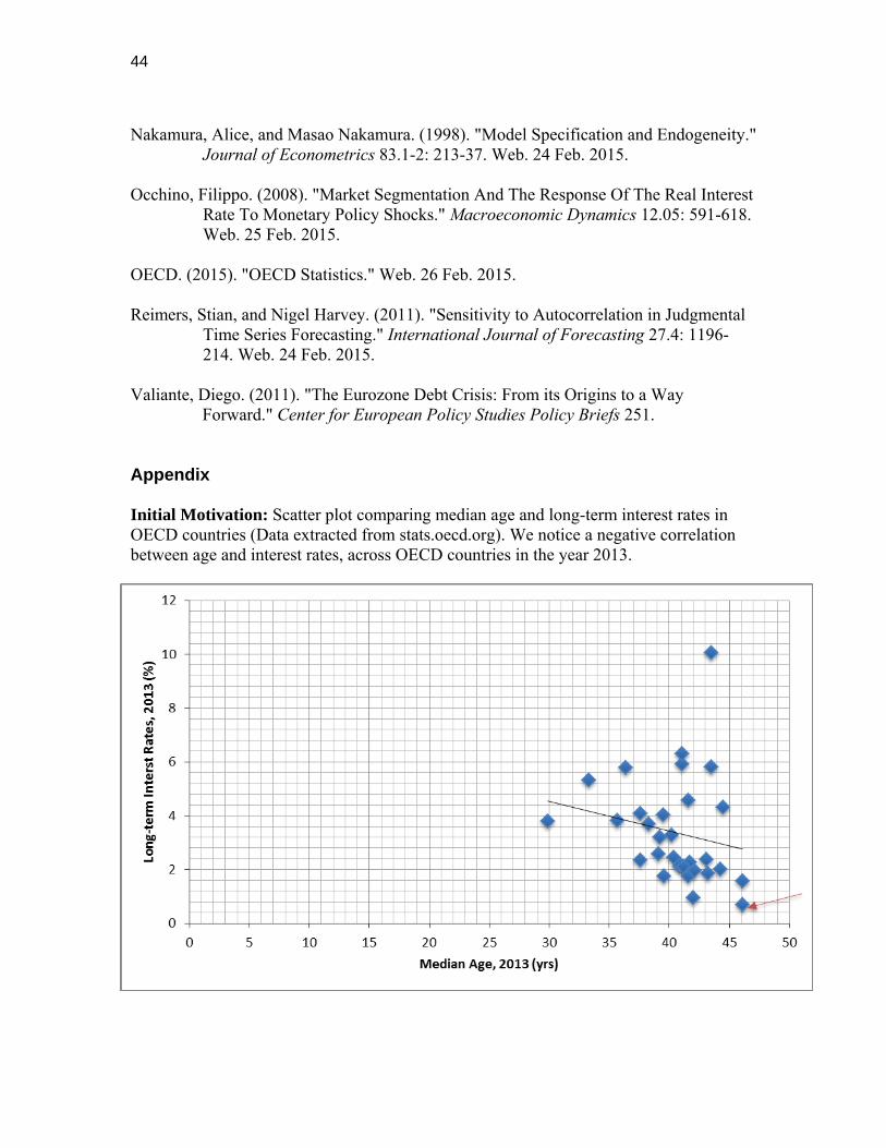
44

Nakamura, Alice, and Masao Nakamura. (1998). "Model Specification and Endogeneity."

Journal of Econometrics 83.1-2: 213-37. Web. 24 Feb. 2015. Occhino, Filippo. (2008). "Market Segmentation And The Response Of The Real Interest

Rate To Monetary Policy Shocks." Macroeconomic Dynamics 12.05: 591-618. Web. 25 Feb. 2015.

OECD. (2015). "OECD Statistics." Web. 26 Feb. 2015. Reimers, Stian, and Nigel Harvey. (2011). "Sensitivity to Autocorrelation in Judgmental

Time Series Forecasting." International Journal of Forecasting 27.4: 1196-214. Web. 24 Feb. 2015.

Valiante, Diego. (2011). "The Eurozone Debt Crisis: From its Origins to a Way

Forward." Center for European Policy Studies Policy Briefs 251. Appendix Initial Motivation: Scatter plot comparing median age and long-term interest rates in OECD countries (Data extracted from stats.oecd.org). We notice a negative correlation between age and interest rates, across OECD countries in the year 2013.

45

Dependent Variables

Stir

Short-term interest rates (3-month interbank offer rate or rate associated with Treasury bills, Certificates of Deposit or comparable instruments).

Termspread The difference between bond yield rates at different maturities.

Variables of interest: Measures of age Medage Median age of the population in each country. Pcpop65 Percentage of the population over 65 years old Dependencyratio The old dependency ratio.

Control Variables Infl The annual inflation rate in a country

Grosssave The gross national income less total consumption, plus net transfers (public)

Exrate The exchange rate for each country expressed in terms of US dollars

Year 1970 - 2015

Countries Countries label, 1 to 34

Grosscapform Gross domestic investment as a percentage of GDP

Curr_acc_bal The sum of net exports of goods and services, net primary income and net secondary income as a percentage of GDP

Lforcegr The rate of growth of the working age population

Govtdebt Domestic and foreign liabilities such as currency and money deposits, securities other than shares, and loans

Riskpre The interest rate charged by banks on loans to private sector customers minus the "risk free" treasury bill interest rate

Stockspcgdp The total value of shares traded during the period, as a percentage of GDP

Fdi The sum of equity capital, reinvestment of earnings, other long-term capital, and short-term capital as shown in the balance of payments

46

Table (a): Number of observations, the range, mean and standard deviation for each variable (1970-2013)

Table (b): Number of missing observations, the number of total observations, and

the proportion of missing observations (1970-2013)

47

Table (c): Number of observations, the range, mean and standard deviation for each variable (1990-2013)

Table (d): Number of missing observations, the number of total observations, and

the proportion of missing observations (1990-2013)

48

Abstract

Information and Communication Technology (ICT) such as the world-wide application of mobile phones and internet have contributed substantially to the fast-growing world economy in unprecedented ways. Our research focuses on the influence of those two technologies and tries to answer the question, “how does ICT influence agricultural output in China?” Through an empirical analysis utilizing panel data from 27 provinces of China across a period of 10 years, our results indicate that in spite of our previous prediction that those two technologies contribute positively to the development of Chinese agriculture, we see negative influence of mobile phones and positive influence of internet. Possible explanations and further discussions are provided. Introduction

Agriculture, known as the primary industry of the modern world, has been experiencing constant development throughout human history and especially rapid changes over the last few decades. For the purpose of this paper, we define “agriculture” as the combination of farming, forestry, animal husbandry and fishery activities according to the definition by the National Bureau of Statistics of China (NBSC) (2013-2012). It is commonly accepted that technology advancements are the keys to a more developed economy. We hence deduce using the same rationale that agriculture development is affected by technological changes as well. A few honorable mentions of such technological changes may be the mechanization of farming equipment, development of multiple-field crop rotation as well as the development of fertilizers in the Green Revolution (Sunding and Zilberman, 2001). While these technological changes were mainly focused on the physical production of crops, livestock or fishery, more recent technological advancements like the introduction of Information and Communication Technology (ICT) emphasize on a broader aspect, including production, transportation, communication, marketing, reproduction and even education. The effects of these ICTs on the world economy have been studied systematically by many scholars but we intend to focus on the effects on the agricultural sector of China which, considering the rising status of China as a world-class economy, received little attention. That might be due to the fact that China has only been experiencing rapid growth for the last few decades and the agricultural sector even more recently. Complete and systematic data are difficult to obtain as a result of the less-developed statistics department of the Chinese government, local and central. For the purpose of this research, we selected two of the most prominent information technology realizations as our observation: internet

49

and mobile phone. A survey conducted in 2014 showed that out of 1.26 billion people in China, 886 million mobile connections have been established which attributes to 405 million mobile subscribers, surpassing the total population of the United States. While the Chinese rural area has been experiencing relatively slow development compared to urban counterparts, on average the rural population actually possess 1.18 SIM cards per person which means everyone is accessible to mobile phone coverage (Gillet, 2014). On the other hand, the internet penetration rate reached 62.8 percent for the urban population in 2014. The rural area however enjoys a much lower penetration rate at 28.8 percent which accounts for 178 million users as for 2014. What’s more interesting is the interaction of mobile phone and internet since 71.3 percent of rural netizens actually access the internet through mobile phone networks (China Internet Network Information Center (CNNIC), 2014). As we can see from Graphs 1.1, 1.2, 1.3, gross output of agriculture, mobile phone ownership and computer ownership all show a similar increasing trend over the decade. Mobile phone and Internet are inevitably two of the most influential and representative ICTs in the early 21st century not only because of their rapid penetration of everyday life, but also the influence on almost every industry. According to Chu (2013), Internet positively impacts the economy since “it spreads information, stimulates innovation, builds up network, fosters business, deepens capital, improves labor market, strengthens market competition, and helps firms to profit from emerging markets.” As the Era of Information dawned on us in the late 20th century, we are curious to find out how much benefit, if any, the information and communications technology would bring to agriculture, the oldest industry in the world and that was our motivation to carry out this research.

The following essay will be arranged as follows: Section 1 gives an overview and discussion of the literature we found pertaining to the effects of ICT on agriculture as well the national economy. Section 2 introduces our empirical model and the methodology we will use to analyze the data we found. Section 3 shows the results on which accordingly we will have our discussion and what could be improved. Section 4 concludes. 1. Literature Review ICT Influence on National Economy

The positive influence of information and communication technology on a country’s economy has been studied thoroughly by many scholars. Early research conducted by Hardy (1980) collected data from 60 nations over a period of 13 years, stating that telecommunication does contribute to economic development and furthermore the contribution comes from the support of telecommunication on the organization of economic activities. He continues to conclude that telecommunication investment showed the largest effect in the least developed countries while the most developed countries received the smallest benefits, which indicates that telecommunication development in countries with less developed infrastructure actually brings more benefits than in developed countries. Fuss et al. (2005) specify by suggesting that mobile phones instead of personal computers are actually the driving force of closing

50

the digital divide between the developed and developing countries (Fuss et al., 2005). Yi and Choi (2009) stated that through their research they found a positive and significant role of internet in the development of a country’s economic growth. Using their empirical model (model 1.1), they utilized a macroeconomic approach with cross-country data controlling variables of investment ratio, government consumption ratio and inflation rate to estimate the effect of the internet on the national economy. Their results show that every 1 percent increase in internet user ratio could lead to a 0.057 percent increase in GDP growth rate. More studies were conducted to determine the influence of ICTs on economic factors. According to Norton (1992), ICT infrastructure significantly lowers the cost of acquiring information and various costs of participating in markets. He further states that it is also plausible to argue that a low telecommunication infrastructure is one reason why some parts of the world have not developed. Röller and Waverman (2001) argue that as ICT infrastructure improves, transaction costs reduce, and output increases for firms in various sectors of the economy. Yet different from the view of Hardy (1980), the authors conclude through their empirical analysis that an increase in telecommunication infrastructure could create higher growth effects in OECD (Economic Co-operation and Development) countries than in the less-developed non-OECD countries. ICT Influence on Agriculture

Thysen (2000) noticed a rather modest use of ICT among farmers and explained by saying that farmers could obtain higher agricultural output by simplification of farming methods and application of cheap externally produced inputs such as fertilizers and pesticide. Nonetheless, the development of ICT and more restriction on use of chemical in agriculture would result in an inevitable decrease in cheap agricultural methods and increase in the application of ICT, which is deemed as sustainable and variable. Some potential ways of an ICT application may be: high precision application of chemicals, caring livestock, food documentation and agricultural extension (which will be discussed later in detail). Some scholars have explored the real-life application of the functions above. McKinion et al. (2004) introduced the wireless local area networking (WLAN) system in the Paul Good Farm in Noxubee County, MS, USA, which wirelessly connected cotton pickers, spray equipment, variable rate fertilized application equipment, and hand-held personal digital assistant computers in the field, allowing for rapid bi-directional movement of data and information. Another survey conducted by Burke and Sewake (2008) focused on the influence of internet on small flower farms in Hawaii, USA. Their results suggested that the internet could potentially boost agricultural sales by presenting the case in which 18 percent of the survey participants saw more than a 75 percent increase of flower sales after their adoption of a computer and an internet network.

Mobile phone technology enjoyed even more attention from researchers because of their widespread application in the world economy, especially the less-developed economies. Many surveys and cross-country analyses have been conducted to determine the effect of mobile phone adoption and application. Sridhar et al. (2007) argues that the average

51

prices of agricultural commodities are higher in villages with access to mobile phones than the ones without. Parker (2005) found that in 2004 there were more new mobile phone subscribers in Sub-Saharan Africa than the whole of North America. Muto and Yamano (2009) found out through their survey in Uganda that mobile phone coverage in the urban and rural areas has a positive and significant influence on prices of agricultural commodities. They also suggested that it was not necessarily the personal possession of mobile phones but the simple expansion of mobile phone coverage in remote areas that increased the prices because the application of mobile phones eliminated the information asymmetry in remote rural areas by giving the farmers the opportunity to find the highest bidders for their commodities. Other research carried out by Mittal et al. (2010) points out that “the introduction of mobile phones decreased price dispersion and wastage by facilitating the spread of information”, which leads to more efficient markets and increased social welfare. They categorize the benefits of mobile phones into: “easy access to customized content, mobility and timesaving or convenience”. They also suggest that despite the acclaimed usefulness of mobile phone application, these benefits would be unevenly distributed between rural population with lacking policy guidance from the government and underdeveloped infrastructure. ICT for Agricultural Extension

Besides the influence of mobile phones and internet on the production and marketing aspect of agricultural output, these ICTs are also implemented to improve the education level of agricultural participants. According to Birhaeuser et al. (1991), agricultural extension services are one of the most common public sector supports of knowledge diffusion, which bridges the gap between discoveries in laboratories and changes in individuals’ farms. Aker (2011) also states that through the so-called “agricultural extension” programs the rural population could gain access to information and knowledge they need in agricultural production by receiving technological advice from experts via newly introduced ICTs. An example would be that they could receive SMS from mobile phones, which are less expensive than landline phones and more ample in content than radio. Some mobile phone applications also address difficult problems by providing complimentary services via the internet network, such as access to credit or savings, or agriculture and health insurance. Besides the knowledge diffusion function, agricultural extension programs also serve as the feedback units for the individuals’ farms, which express their concerns and questions to the public agencies (Birhaeuser et al., 1991).

Empirical Models in the Literature

We found several articles containing empirical models about the relationship between national GDP or agricultural output (level or growth) and ICTs. One is by Shenggen and Zhang (2004) (model 1.2). They constructed this model to estimate the influence of infrastructure like road (ROADS), percentage of irrigated area in total cropped area (IR), research and development staff (RD), education level (SCHY) and number of rural telephone sets per

52

thousand rural residents (RTR) on both agricultural and non-agricultural outputs. The simultaneous equation system eliminates the potential endogenous problems present in the agricultural production function, in which the first equation represents the influence of variables like land (LAND), agricultural labor force (AGLABOR), fertilizer (FERT), machinery (MACH) on agricultural output (AY) and the second equation the influence of electricity, road, etc. on non-agricultural output (NAY) represented by the gross value of the township and village enterprises (TVE)1. This model inspired us since it utilized a simultaneous equation system where the variables of concern were used to estimate outputs of agricultural and non-agricultural sectors in rural areas, which was designed to eliminate the endogeneity problem. We encountered similar problems in our research. Another model was presented by Lin (1992) (model 1.3), where in equation (1) the author uses variables land, labor, capital, chemical fertilizer (Fert), the index of market prices relative to manufactured input prices (MP), the index of above-quota prices relative to manufactured input prices (GP), the percentage of total sown area in non-grain crops (NGCA) (we used cultivated land area in our research instead since sown land area potentially overestimates the land cultivated because of multiple cropping), the multiple cropping index (MCI), ratio of households converted to Household Responsibility System (HRS), and a time trend (T) to study the influence of HRS on the rural economy. Similar to the previous model, this model utilized some common factors like land, labor, capital and fertilizer while introducing some more problem-specific variables to estimate the influence of HRS. 2. Methodology

We built our own empirical model on those presented above in the literature review (model 2.1). The data set used for our study was collected by the National Bureau of Statistics of China (NBSC, 2003-2012) which possesses governmental authority and credibility (table 2.1). The data set includes individual data for 27 selected provinces across China for the time period of 2003-2012, which gave us 270 observations for each variable for the panel data (some missing values are present). Our variables include gross output value of farming, forestry, animal husbandry and fishery (Y), sown land area (Land)2, number of rural employed persons in farming, forestry, animal husbandry and fishery (Labor), consumption of chemical fertilizer (Fertilizer), major agricultural machineries (Machinery), number of mobile phones owned per 100 rural households (Mobile) and number of computers owned per 100 rural households (Computer). The choice of which variables to include in our study was largely affected by the availability of data. The year 2003 is set as our base year since NBSC only provided data for the number of computer

1 Township and Village Enterprises (TVE) are market-oriented public enterprises mostly in the secondary sector, under the purview of local governments based in townships and villages in the People's Republic of China. 2 Cultivated land area would have been a better choice since it eliminates the possibility of multiple cropping in agricultural practices but once again, we were unable to obtain credible data from credible sources for this variable.

53

ownership in rural areas starting from then. Based on our previous investigation, the number of SIM card subscribers and internet users are preferred in representing the penetration of mobile phones and internet. Nevertheless, through our search for the data, neither provincial level data nor rural area data were reachable for us. We then took an alternative route by using the data of total quantity of mobile phones and that of computers possessed by rural households in our study. In this analysis, Beijing, Tianjin, Shanghai, Chongqing, Hong Kong and Macau were considered outliers and not included in our data set due to their special status and relative lack in agricultural activity engagement. For the rest 27 provinces, we obtained their gross output values of farming, forestry, animal husbandry and fishery of each year, and calculated the real gross output values by deflating the nominal values by agricultural product price indices (Base year=2003). The number of employees in the corresponding sectors in rural areas was available and directly used in our study. Machinery here is represented by the total power (in 10000 kW) consumed at the end of each year. Volume of the effective component of chemical fertilizer is measured in 10000 tons and is the sum of Nitrogenous fertilizer, Phosphate fertilizer, Potash fertilizer and Compound fertilizer. Land area is the total sown areas of farm crops in 1000 hectares. The levels of mobile phone and computer ownership were obtained by multiplying the number of mobile phones or computers owned per 100 rural households by the number of rural households and divided by 100. To eliminate the potential time-invariant errors and obtain robust estimates for data that is collected in the same way and from the same sample group, fixed effect estimation is preferred to random effect estimation (Borenstein et al., 2010). Also, from the results we could see that random effect estimation gave exactly the same numbers as the standard OLS regression. As we learned from the literature survey, there exist potential endogeneity problems between the mobile phone penetration rate and the error term. Also, feedback could be present in our model since we cannot determine the causality between agricultural output (in terms of real income) and mobile phone ownership (Graph 2.1, 2.2). We opt for a two-stage least square model in hope of eliminating this feedback effect as well as the potential endogeneity problems between variables Mobile and the gross output values of the agriculture sector. The choice of instrument variable was a challenge for us because of the insufficient data problem mentioned above. We tried to use variables like the research and development (R&D) expenditure, prices of mobile phones, gross output of TVEs, etc. None of them showed the capability as a potent IV. Based on our research, we then picked the total enrollment in tertiary education (regardless of age, expressed as a percentage of the total population of the five-year age group following on from secondary school) as the instrument variable. The data we obtained on Tertiary was collected by the World Bank (2003-2012). Despite the missing data in 2003 and 2004, the school enrolment rate of tertiary education works well as an instrument variable since it shows high correlation with Mobile and low correlation with Y. The coefficient of log(Mobile) (-1.10), however, is unreasonably large and negative, which lacks economic significance. Furthermore, although the variable tertiary showed promising candidacy as an IV, the

54

data were collected from the national level instead of the provincial, rural level which does not fit into our research framework perfectly. After consideration, the second instrumental variable we used was the mobile phone penetration rate of urban areas for the corresponding provinces we studied in the same time period. This instrumental variable gave us better results and is included in our final model. 3. Results and Discussion

Results are shown in table 3.1. We first ran OLS regression with the total number of mobile phones and computers owned by the rural households and found the estimate for mobile phones was not significant (indicated by OLS*). The output we obtained by running OLS regression to our structural equation with the penetration rates of mobile phones and computers, however, indicated that both of these two variables have significant influences on our dependent variable. The explanation for the differences in these two results could be that it is the penetration rate instead of the level of mobile phones and computers that determines the change in agricultural output values, which aligns with the conclusion of a previous study by Muto and Yamano (2009). The fixed effect estimation shows very similar results to the OLS, which suggests that there did not exist significant time-invariant errors and the OLS results are already quite robust. The first stage of our two-stage least squares estimation showed a significant influence of the mobile phone penetration rate in urban areas on the growth rate of mobile phone penetration rate in rural areas and the R-square of the first stage regression was 0.8310, both indicating that Urban is a good instrument variable here. The second stage output did give us a significant estimate of -0.066 on log(Mobile), that is, with a 1 percent increase in the number of mobile phones, the gross output values of agriculture sector decrease by 0.066 percent. This result, however, does not match our assumption that the increasing penetration of mobile phones will boost gross agricultural output. The unexpected negative estimate of log(Mobile) could be explained in a few ways. Based on the literature we reviewed, though Chinese rural population have good access to mobile phones and related infrastructure, they mainly use mobile phones for entertainment or daily communication, which does not have much involvement with agricultural activities. Also, according to a previous study by Abraham (2006), instant information has greater influence on perishable goods than non-perishable goods in terms of market prices. In China, rice, wheat and corn are the major planted crops and the market prices of these products might not be significantly affected by faster access to market information, thus no positive impact on the gross output values. Another reason for increasing mobile phone penetration hampering agricultural output could be that with access to more opportunities, people in rural areas might leave farmlands and turn to other businesses, especially TVEs that have been rapidly established across Chinese rural areas. Taking into account the cultural background of China that rural households are

55

eager to leave the countryside and get their “Hukou1” transferred to urban cities, there is a greater chance of participants in the agriculture sector leaving farmland and seek more profitable jobs with more information provided (Chan and Zhang, 1999). In order to corroborate this hypothesis, we tried to use the variables like migration population to estimate the agricultural output but the data for migration population only started being recorded from 2012, in quarters and at the national level, which is incompatible with the other variables we have. Another challenge we encountered in the analysis was to determine the usefulness of the variable Land, which is controversial to be included in the model. We took the data on sown areas of farm crops, which is only related to the farming sector. No data equivalent to land areas could be obtained to explain variation in the change of gross output values due to other sectors of agriculture, namely animal husbandry, forestry and fishery. Although data for the areas of orchard or aquaculture area are available, there are too many missing values in the data set and considered to hamper the significance of the variables. Empirically, the OLS results showed that the variable Land does not have statistical significance in our model. Since we tried to limit our area of study to the agriculture sector only, we have been encountering similar problems when carrying out the study due to the insufficient data we could obtain from credible sources, especially the NBSC. 4. Conclusion

Information and communications technology has induced great changes to the modern world. China, as one of the most rapidly developing countries, undoubtedly has also benefited from the introduction of ICT in many different ways. We are curious whether or not these changes also apply to the agriculture sector which is known to be labor-intensive and suffers low total factor productivity. We used two variables of concern, mobile phone and computer, to estimate the influence of mobile phone and Internet penetration rates on the agricultural output of rural China. By running an IV regression, we found that there are significant relationships between mobile phone and agricultural output as well as computer and agricultural output. While the latter one exhibits a positive relationship, as we predicted, the former one contradicts our hypothesis by showing a negative relationship. Although this result took us by surprise, we did find strong evidence supporting it from our extended literature review. One survey from CNNIC suggests that mobile phones in rural China are generally used for entertainment instead of an agricultural purpose. Studies by Chan and Zhang (1999) also suggest that with the introduction of ICT in rural China, agricultural participants would choose to leave the farmlands and look for more lucrative jobs in cities, which actually drags down the agricultural production. We intended to corroborate these statements by running our own regressions but due to the lack of data from the NBSC and other credible sources, we were unable to obtain a robust conclusion. Nonetheless, our result

1 A hukou is a record in the system of household registration required by law which officially identifies a person as a resident of an area and includes identifying information such as name, parents, spouse, and date of birth. This system is criticized for its entrenchment of social strata, especially as between rural and urban residency status.

56

and other literature all lead to the same point: while ICT is known to bring positive changes across the world, some part of it does not empirically benefit the agricultural sector as we expected. This conclusion is as interesting as it is troubling since we are now faced with more questions that need solving in the future. How can we exploit ICT to reap the most benefits for the agricultural sector? Or is it beneficial to keep developing ICT in rural areas when there are more cost-effective methods available? With more focus on high-quality agricultural development in the recent years and hopefully more established statistical departments within the Chinese government, we might be able to solve these questions for China, and even the world economy. References Abraham, Reuben. (2006). "Mobile Phones and Economic Development: Evidence from

the Fishing Industry in India." In Information and Communication Technologies and Development. ICTD'06. International Conference on, pp. 48-56. IEEE, 2006.

Aker, Jenny C. (2011). "Dial “A” for Agriculture: A Review of Information and

Communication Technologies for Agricultural Extension in Developing Countries." Agricultural Economics 42, no. 6: 631-647.

Birkhaeuser, D., Evenson, R. E., and Feder, G. (1991). “The Economic Impact of

Agricultural Extension: A Review.” Economic Development and Cultural Change, 607-650.

Borenstein, Michael, Larry V. Hedges, Julian Higgins, and Hannah R. Rothstein. (2010).

"A Basic Introduction to Fixed‐effect and Random‐effects Models for Meta‐analysis." Research Synthesis Methods 1, no. 2: 97-111.

Burke, Kelly, and Kelvin Sewake. (2008). "Adoption of Computer and Internet

Technologies in Small Firm Agriculture: A Study of Flower Growers in Hawaii." Journal of Extension 46, no. 3.

Chan, Kam Wing, and Li Zhang. (1999). "The Hukou System and Rural-urban Migration

in China: Processes and changes." The China Quarterly 160: 818-855. Choi, Changkyu, and Myung Hoon Yi. (2009). "The Effect of the Internet on Economic

Growth: Evidence from Cross-country Panel Data." Economics Letters 105, no. 1: 39-41.

Chu, Shan-Ying. (2013). "Internet, Economic Growth and Recession." CNNIC. (2014). 35th Statistical Report. CNNIC Statistical Reports. Fuss, Melvyn, Meloria Meschi, and Leonard Waverman. (2005). "The Impact of

Telecoms on Economic Growth in Developing Countries in Africa: The Impact of Mobile Phones." Vodafone Policy Paper Series no 2.

57

Gillet, J. (2014). “Measuring Mobile Penetration: Untangling 'Subscribers', 'Mobile Phone Owners' and 'Users'”, GSMA Intelligence Research Notes.

Hardy, Andrew P. (1980). "The Role of the Telephone in Economic Development."

Telecommunications Policy 4, no. 4: 278-286. Lin, Justin Yifu. (1992). "Rural Reforms and Agricultural Growth in China." The

American Economic Review 34-51. McKinion, J. M., S. B. Turner, J. L. Willers, J. J. Read, J. N. Jenkins, and John McDade.

(2004). "Wireless Technology and Satellite Internet Access for High-speed Whole Farm Connectivity in Precision Agriculture." Agricultural Systems 81, no. 3: 201-212.

Mittal, Surabhi, Sanjay Gandhi, and Gaurav Tripathi. (2010). “Socio-economic Impact of

Mobile Phones on Indian Agriculture.” New Delhi: Indian Council for Research on International Economic Relations.

Muto, Megumi, and Takashi Yamano. (2009). "The Impact of Mobile Phone Coverage

Expansion on Market Participation: Panel Data Evidence from Uganda." World Development 37, no. 12: 1887-1896.

National Bureau of Statistics of China. (2003-2012).

http://www.stats.gov.cn/english/Statisticaldata/AnnualData/ (accessed 3 9, 2015). Norton, Seth W. (1992). "Transaction Costs, Telecommunications, and the

Microeconomics of Macroeconomic Growth." Economic Development and Cultural Change. 175-196.

Parker, S. (2005). "Wireless Technology Helping to Shrink Digital Divide." Voice of

America, May. http://www. voanews. com/english/2005-05-06-voa57. cfm.(accessed August 12, 2005).

Röller, Lars-Hendrik, and Leonard Waverman. (2001). "Telecommunications

Infrastructure and Economic Development: A Simultaneous Approach." American Economic Review. 909-923.

Shenggen, F. A. N., and Xiaobo Zhang. (2004). "Infrastructure and Regional Economic

Development in Rural China." China Economic Review 15, no. 2: 203-214. Sridhar, Kala Seetharam, and Varadharajan Sridhar. (2007). "Telecommunications

Infrastructure and Economic Growth: Evidence from Developing Countries." Applied Econometrics and International Development 7, no. 2.

58

Sunding, David, and David Zilberman. (2001). "The Agricultural Innovation Process: Research and Technology Adoption in a Changing Agricultural Sector." Handbook of Agricultural Economics 1: 207-261.

Thysen, Iver. "Agriculture in the Information Society." (2000). Journal of Agricultural

Engineering Research 76, no. 3: 297-303. World Bank. (2003-2012).

http://databank.worldbank.org/data/reports.aspx?source=2&country=CHN&series

=&period= (accessed 3 9, 2015).

Appendices Model 1.1:

0 1 2 3 4it it it it it itGrowth Internet Investment Government Inflation u

Model 1.2:

AY = f(LAND, AGLABOR, FERT, MACH, IR, RD, SCHY, ROADS, RTR), NAY = f(RILABOR, ELEC, SCHY, ROADS, RTR). Model 1.3:

1 2 3 4 5

6 7 1 8 9 10 11

39

12

(1) it it it it it

it t t it it t

j j itj

ln Y a a Land a ln Labor a ln Capital a ln Fert

a HRS a MP a GP a NGCA a MCI a T

a D e

331 2 3 1 4 5 ( 6)( (2) )it it t t t i itln Y HRS b MP b GP T iDi

Model 2.1

0 1 2 3

4 5 6

it it it it

it it

logMobile b b log Labor b log Machinery b log Fertilizer

b log Land b log Urban lo

0 1 2 3

4 5 6

it it it it

it it it it

logY log Labor log Machinery log Fertilizer

log Land log Mobile log Computer

59

Table 2.1 Data Summary

Variable N Mean St. Dev Min Max

Y 261 1339.5 837.0 58.6 3870.9 (in 100 million yuan) Mobile 270 102.0 64.6 2.3 244.5 (number of mobile phones per 100 households) Computer 264 6.5 8.9 0.1 47.9 (number of computers per 100 households) Labor 270 1035.4 704.9 84.4 3321.2 (in 10000 persons) Machinery 270 2909.5 2645.9 181.2 12419.9 (in 10000 kw) Fertilizer 270 186.0 135.1 3.19 684.4 (in 10000 ton) Land 270 5641.9 3435.7 231.2 14262.2 (in 1000 hectare)

Source: CNNIC

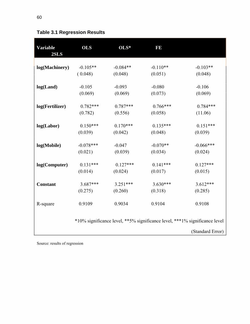
60

Table 3.1 Regression Results

Variable OLS OLS* FE 2SLS log(Machinery) -0.105** -0.084** -0.110** -0.103** ( 0.048) (0.048) (0.051) (0.048) log(Land) -0.105 -0.093 -0.080 -0.106 (0.069) (0.069) (0.073) (0.069) log(Fertilizer) 0.782*** 0.787*** 0.766*** 0.784*** (0.782) (0.556) (0.058) (11.06) log(Labor) 0.150*** 0.170*** 0.135*** 0.151*** (0.039) (0.042) (0.048) (0.039) log(Mobile) -0.078*** -0.047 -0.070** -0.066*** (0.021) (0.039) (0.034) (0.024) log(Computer) 0.131*** 0.127*** 0.141*** 0.127*** (0.014) (0.024) (0.017) (0.015) Constant 3.687*** 3.251*** 3.630*** 3.612*** (0.275) (0.260) (0.318) (0.285) R-square 0.9109 0.9034 0.9104 0.9108

*10% significance level, **5% significance level, ***1% significance level

(Standard Error)

Source: results of regression

61

Graph 1.1

Graph 1.2

62

Graph 1.3

Graph 2.1

63

Graph 2.2

64

Abstract

This paper uses time-series analysis techniques to examine the wealth effects of the stock market in the US over the period 1952 to 2014. The data used in this paper are from the Federal Reserve Bank of St. Louis (FRED). To separate the wealth effects of the stock market from other forms of wealth, the total wealth of households are divided into stock wealth and non-stock wealth. Three aspects of the wealth effects of the stock market are analyzed in this paper: how large are the wealth effects, how fast do households adjust to the wealth effects and are the wealth effects stable over this long period? By applying a cointegration test, this paper finds a long-run relationship between consumption, income and wealth. However, the estimated error correction model (ECM) suggests that the fluctuations in the stock market will not affect consumption in the short-run. The results of ECM also show that households will adjust their consumption in the short-run in order to restore their long-run equilibrium level. Nevertheless, the adjustment speed is found to be quite slow. In the last section of this paper, several potential issues about quantifying the wealth effects of the stock market are discussed and some suggestions for future studies are given.

Acknowledgments

I would like to thank professors Desmond McKeon and Özden Sungur for their advice during the process of writing this paper. I would also like to thank my parents for their continued support when I am studying abroad. China Scholarship Council gives me financial support to study abroad and I am very grateful for it. Introduction

In the last two decades we have seen a dramatic expansion of the US economy. According the Bureau of Economic Analysis of the US (2016), the consumption expenditure per capita has increased from 15082 dollars in 1990Q1 to 37600 dollars in the 2015Q1; about 250 percent as much as the consumption in 1990. Meanwhile, the stock market also experienced a huge increase. Fluctuations in the stock market have profound effects on the economy. During the 1990s, the stock market boom greatly increased the average family’s wealth and stimulated consumption in the US. The wealth effect of the stock market is an interesting economic research topic and has motivated numerous studies to quantify its scale. In this paper, I also seek to investigate how fluctuations in the stock market will affect the consumption of households.

65

There are two different aspects of the wealth effects of the stock market. The first one is how much a representative consumer will spend given a one-dollar appreciation in his/her portfolio. Due to the volatility of the stock prices in the short-run, households may not consider the appreciation of their stock portfolios to be sustainable. What’s more, the existence of commission, capital gains tax and other transaction costs might prevent the household from cashing his/her portfolios. They might also prefer to hold the portfolio for a longer time, hoping for further appreciation in their portfolios. Therefore, there are many different forces affecting the wealth effects of the stock market simultaneously. The second aspect of the wealth effects is to see how fast the average households will adjust to the changes in their stock wealth. Due to adjustment costs, the changes in the wealth effects will not affect the consumption level of households all at the same time. There might be time lags for people to realize the appreciation of their stock portfolios. In addition, it also takes time for households to decide what they want to buy. Therefore, it is important to investigate whether the stock market has long-lasting effects on the consumption of households. Most of the previous literature has focused on evaluating the scale of the wealth effects on consumption. This paper makes some additional contributions by investigating both the how large the wealth effects of stock market are and how fast households will adjust to the changes in their stock wealth. By setting a restriction on the coefficients of the regression, I am able to estimate the long-run multiplier as well as the adjustment speed of the wealth effects of the stock market. Previous literature has suggested that none of consumption, income and wealth is a stationary process and each contains a unit root process. Traditional ordinary least square methods might bring about some problems like the non-normal distribution of the estimators. However, in this paper I use the residual based cointegration test to investigate if these three variables share a same stochastic trend in the long run. If consumption, income and wealth are cointegrated, then the OLS estimator of the marginal propensity to consume out of wealth will be “superconsistent”. Then I analyze the short-run wealth effects of the stock market on consumption using the error correction model (ECM). I find that the fluctuations in the stock market do not contribute to the changes in consumption. The reason for this is not that the stock market does not have wealth effects on consumption, but fluctuations in the stock market in the short run are usually transitory. This paper is divided into six sections. The following literature review provides the theoretical background of this paper as well as other previous empirical studies. The data and variables section provide information about the source of the data used in this paper and how each variable is defined. In the model and methodology section I derived the models that will be applied in this paper. The empirical results section presents the statistical results of these models and some explanation. The last part is conclusion and discussion, where I make a brief conclusion and present some final thoughts about the choice of model and some potential problems.

66

Literature Review Theoretical Linkage Between Stock Market Wealth and Consumption

Various economic theories have suggested the potential relationship between wealth and consumption. Among them, the two most frequently used models are Friedman’s permanent income hypothesis and Modigliani’s life-cycle model. According to the life-cycle model, the current level of consumption is determined by income and the level of total wealth. The increase of consumption in response to a one-dollar increase in wealth is called the marginal propensity to consume out of wealth. Stock equity is an important part of the total wealth that households hold and therefore, an increase in the stock market should spur households to consume more. However, in light of Friedman’s permanent income hypothesis, income is divided into two parts-permanent income and transitory income. Between them, only changes in permanent income will significantly affect consumption. Changes in transitory income will only slightly affect consumption because households will try to smooth their consumption through saving and borrowing. For example, if a man lost 100 dollars on the way home, he will not change his consumption patterns because he knows this change in his income is just transitory: he will not lose 100 dollars every day. However, if there is a recession and his salary is decreased by 100 dollars every week, he might try to tighten his belt because this change has affected his permanent income. Since the fluctuations in the market value of stock are usually considered as transitory, the permanent income hypothesis argues that the wealth effects of the stock market will be relatively small. Therefore, according to these two theories, the marginal propensity to consume (MPC) out of the stock market wealth will be positive, but relatively small.

Empirical Linkage Between Stock Market Wealth and Consumption

A considerable amount of research has been done to examine the relationship between wealth, income and consumption. Most of this research found a significantly positive but small value of the MPC out of stock wealth. The value of MPC is between 0.03 and 0.08, which suggests that the household will consume three to eight cents in response to a one-dollar increase in stock market wealth. But, the MPC seems to vary over time. These changes in the MPC will be explained in more detail in the latter part of this paper.

Macklem (1994) divided wealth into two parts: human wealth and non-human wealth, where human wealth is just a measure of education, health etc. and non-human wealth includes wealth in the form of financial assets like equity and other non-financial assets like real estate etc. Using an error correction model (ECM), he found that the consumption of non-durable goods and services will increase by 3.5 cents for one-dollar increase in non-human wealth for Canada. The reason for not including durable goods into consumption is that the consumption of durable goods usually represents additions and replacements to the capital asset, which has different incentives with the consumption of non-durable goods and services. Pichette (2004) used a similar methodology and estimated the long-run MPC out of stock wealth to be 0.02 for Canada.

67

He separated the stock wealth and real estate wealth, and found that changes in house prices have stronger wealth effects on consumption than changes in stock prices. The reason for this difference is that housing wealth is less concentrated among the richest people than stock wealth, and changes in house prices are less likely to be reversed than stock prices. Ludvigson and Steindel (1999) estimated the MPC out of stock wealth for the US. Using an updated approach, they found that the MPC for the US is about 0.046. One interesting fact they found is that the MPC out of stock wealth seems to be unstable across different time periods, with the MPC to be much lower in the 1990s when the economy was experiencing an economic bubble. In the short run, the results of the Granger causality tests are very insignificant and therefore the fluctuations in the stock market do not change the consumption level of households. Though the number 0.046 looks small, when multiplied by trillion-dollar fluctuations of the stock market the wealth effects are considerable even compared with the whole economy. Using panel data for 16 OECD countries, Ludwig and Sløk (2004) found that the long-run MPC out of stock wealth to be ranged from 0.015 to 0.05 in these countries. However, the short-run MPC is much smaller compared with the long-run MPC, which indicates that the stock market plays a less important role in the short run. Data and Variable

The data used in this paper are from Federal Reserve Bank of St. Louis (FRED). As is shown in the literature, durable goods are usually excluded when analyzing the wealth effects of stock market because the incentives for the consumption of durable goods are different from that of non-durable goods and services. However, I am still very interested in estimating the overall wealth effects on total consumption expenditures so use the total consumption expenditure as the consumption variable used in this paper.1 The first independent variable is disposable income, which measures how much income the households have after accounting for taxes. The second independent variable is total wealth. I use the net worth of households for the total wealth because the net worth equals the total assets of the household minus his/ her total liabilities and correctly captures the definition of wealth. The total wealth is then divided into two parts, stock wealth and non-stock wealth. The stock market wealth is measured by the total market value of corporate equity held by households.2 I use the difference of total wealth and stock wealth for the non-stock wealth. The reason for using the difference of total wealth and stock wealth is that non-stock wealth incorporates all the other forms of asset except stock, including both non-financial assets like real estate and other forms of financial assets like bonds and bank deposits. Therefore, it will be incomplete if I just use the data about some certain types of assets. All of these data have been adjusted to 2009 US dollars so the influences of the price level changes are eliminated. The data are from 1952Q1 to 2014Q4 and are divided into several subperiods because I want to examine whether there are any structural changes during this long period.

1 The consumption data used is consumption expenditure per capita, which includes the consumption of durable goods, non-durable goods and services. 2 The stock wealth is described as the amount of corporate equities held by households in the dataset.

68

The Model and Methodology The Wealth Effects on Consumption: Koyck Model Approach

According to the permanent income hypothesis and lifetime-cycle model, income and wealth both affect the level of consumption. Therefore, the traditional linear aggregate consumption function takes the following form:

0 1 2 3t t t t tC PI SW NSW u (1)

where tC is the consumption at the current period, tPI is permanent income at the

current period; tSW is the stock market wealth and tNSW is non-stock wealth which

could include real estate and other forms of financial assets. tu is the error term that

captures the effects of other effects on consumption. In some literature tu is also called

transitory consumption because it measures the transitory disequilibrium consumption from its equilibrium level. Due to the unobservability of the permanent income, there is a need to modify the consumption function and replace the permanent income with some variables that can be observed. A commonly used replacement for the permanent income is the current disposable income. Suppose wealth and income has a long-lasting effect on consumption. This is plausible because households want to smooth their consumption across different time periods. For example, if one’s portfolio appreciates by ten thousand dollars in period t, this will affect his/her consumption not only in period t but also in the following periods t+1, t+2 etc. Furthermore, suppose that the effects of a change in current income or wealth on consumption attenuate at a rate λ. This means that after one period the

effects will be λ as much as the last period. If the attenuation rate is less than 1, the effects of a change in current wealth in the future will be 0 at last. This restriction on the parameter is plausible since the effect of a change in the distant past on the current period will not be as important as a change in the current period. Given the above two assumptions, the model specification is as the following:

0 1 2 31 1 1

i i it t i t i t i ti i i

C PI SW NSW u

(2)

At first glance, it is not possible to estimate equation (2) because there are infinite parameters needed to be estimated. However, if we lag (2) by one period and multiply it by the attenuation rate λ, we can get

1 1 11 0 1 1 2 1 3 1 11 1 1

λ λ i i it t i t i t i ti i i

C PI SW NSW u (3)

If we subtract (3) from (2) we can get

69

1 0 1 2 3

0 1 1 2 3

λ

λt t t t t t

t t t t t t

C C PI SW NSW v

C C PI SW NSW v

(4)

where 0 0 1 λ and 1λt t tv u u .

Equation (4) is called the Koyck model, which was first proposed by Koyck in 1954. Though the Koyck model is essentially just a simple first-order autoregressive regression, it is a very powerful tool. By applying restriction to the parameters we can get a lot of useful information about the dynamics of the wealth effects of stock market on consumption in the long-run. β1, β2 and β3 are just the impact effects on the consumption. To acquire the long-run cumulative dynamic multiplier of the stock wealth ( )swl , we need

to add up the following geometric series:

2 22 2 2λ

1 λswl

(5)

The same procedure can be applied to income and non-stock wealth to get the long-run multipliers of them. Another usage of the Koyck model is that we can get the adjustment speed of consumption in response to changes in income and wealth. The median lag is the time required for the first half, or 50 percent, of the total changes in the dependent variable following a unit sustained change in the independent variable. For the Koyck model, the median lag is as follows:

log 2median lag

log λ (6)

The lower the attenuation rate λ, the faster the adjustment will be and the lower the

median lag which means that it takes less time to accomplish the first 50 percent of the total change. The Wealth Effects of Stock Market on Consumption: Error Correction Model Approach

Though the Koyck model can give us much useful information about how stock wealth affects households’ consumption, it neglects some potential short-run deviation of consumption from the long-run trend. The long-run dynamic multipliers in the Koyck model tell us how changes in wealth will affect the consumption in the long run, but in the short run the wealth effects might be quite different. What’s more, it has been widely recognized that all of the above variables (consumption, income and wealth) follow deterministic and stochastic trends. This means that these variables are nonstationary and might cause problems to the OLS estimators. The unit root test in the next part will show that each variable contains a unit root and is integrated of order one, I (1), which means

70

that the series itself is not stationary but its first difference is. Returning to equation (2), if consumption, income and wealth are all integrated of the same order, then we can investigate if they share a same stochastic trend. If they do, then they are said to be cointegrated. A simple way to examine the cointegration between them is to check if the error term tu

is stationary. The stationarity of error term indicates that there is a long-run relationship between these variables because though they each contains a unit root and is non-stationary, they never drift too far from each other. It seems like there is an intangible economic force that will drive the variables back from the disequilibrium level. The cointegration between consumption, income and wealth reveals the long-run relationship among them. The error term:

0 1 2 3t t t t tu C PI SW NSW

is also called the equilibrium error because it measures the deviation of consumption, income and wealth from the long-run cointegration relationship. The long-run relationship is about the equilibrium relationship between these variables. However, the relationship between consumption, income and wealth can be more complicated in the short run. The household might not correctly estimate his/her income or total wealth because it is very difficult for ordinary people to accurately estimate his/her income and wealth. What’s more, an emergency might cause the household to spend a large amount of money in the current period but we have reasons to believe that the household will tighten his/her belt in several following periods. Therefore, the deviation of the consumption from its long-run trend in the current period should be alleviated in future periods. A good and commonly used model to estimate the short-run relationship between time series variables is error correction model (ECM). According to the Granger representation theory, if several variables are I(1) and cointegrated, then there is an error correction representation between these variables:

0 1 1 2 3t t t t t tC a Z PI SW NSW e (7)

where 1 1 1 0 1 1 2 1 3 1t t t t t tZ u C PI SW NSW .

This is the error correction model (ECM) and it can tell us the short-run relationship between consumption and wealth. The variable Z is the error correction term, which measures the short-run deviation of the consumption from its long-run equilibrium level in the previous period. The expected sign of 0 is negative. If 1tZ is positive, which

means that the consumption in the last period is higher than its equilibrium level, the product of 1tZ and 0 will be negative. Therefore, the error correction term will push

consumption back towards its long-run equilibrium level. The higher the error correction coefficient 0 is in absolute value, the faster the adjustment process. However, the error

71

correction term Z is unknown so it cannot be used directly in the error correction model and has to be estimated first. A simple and commonly used method is the Engle-Granger two-step procedure: first run a regression of consumption against income and wealth to acquire the cointegration coefficients and equilibrium error, and then use the estimated equilibrium error to run the second regression of the error correction model to get the short-run dynamic relationship. One problem associated with this approach is that the statistical inference about these variables cannot be carried out using the conventional t-statistics because these coefficients do not follow normal distribution even in a large sample. Therefore, some correction is needed to modify the conventional OLS estimators. Here, I adopt the dynamic OLS procedure (DOLS), which was first proposed by Stock and Watson (1993). The dynamic OLS specification for our consumption function takes the following form:

0 1 2 3 1 2

3

k k

t t t t i t i i t ii k i k

k

i t i ti k

C PI SW NSW PI SW

NSW v

(8)

By adding the leads and lags of the first difference of the independent variables, the dynamic OLS estimators are asymptotically normally distributed. Therefore, the standard statistical inference can be carried out here. One issue arises in the course of the estimation for the consumption. The permanent income cannot be directly observed. A simple approach I will follow in this paper is to assume that the permanent income is proportional to the current disposable income. This is reasonable because households cannot directly observe their lifetime income so they have to make rational expectations about their lifetime income based on the information that they have in the current period. By replacing PIt=αDIt with the permanent income in (7) and (8) we can now estimate the effects of income on consumption. Empirical Results Koyck Model

Table 1 shows the regression results for the Koyck model. Data are divided into three subperiods. The reported standard errors in the parentheses are heteroskedasticity and autocorrelation consistent standard error (HAC) because in time series data serial correlation is very common. Therefore, using a HAC standard error to account for that correlation, column (1) shows the coefficients for the whole 1952-2014 period. The attenuation rate λ, which is the slope coefficient of the lagged consumption 1( )tC , is

0.829. The long-run multiplier is calculated by equation (5), which adds up the geometric series of the impact of the variable on consumption. The long-run multiplier of stock wealth is 0.057. Households will consume roughly six cents for every one dollar earning in the stock market. Though six cents is a small number, when multiplied by trillion-dollar fluctuation in the stock market, the wealth effects are still considerable. This value is in line with previous literature. The long-run multiplier of income is 0.85, indicating

72

that households will consume 85 percent of their income. Using equation (6) mentioned in the methodology, we can get the median lag for the wealth effects of the stock market on the consumption. The median lag equals to 3.7, which means that it takes 3.7 periods to complete half of the wealth effects of the stock market on consumption. Considering that quarterly data are used here, 3.7 periods is about one year, indicating that the adjustment speed of the households is quite slow.

Columns (2) to (4) show the regression results for three subperiods. It seems that the wealth effects of the stock market are very sensitive to the estimation period. This instability can be explained by the changes in economic regulation, policy and technology. It can be seen that before 1985 the wealth effects of the stock market is significantly lower than those in the 1990s and 2000s. A plausible reason for this is that before the 1980s, computers and the internet were not as popular as they are today and therefore financial markets are also less popular among households. They are not able to keep track of the fluctuations of the stock market every second as we can today. Only a small portion of households hold stock equity and consequently the wealth effects of stock market are also less significant. The marginal propensity to consume out of stock wealth rises to 0.094 during the 1990s. This can be explained by the stock market boom during that period. As we know, the US economy experienced an economic expansion as well as a stock market boom during 1990s. The stock market was surging and households were willing to invest in stock. According to Hong et al. (2004), 48.9 percent of American households owned stock, either directly or indirectly through mutual funds in the 1990s. However, the participation rate in the stock market was merely 31.6 percent in the 1980s. Therefore, the higher the stock market participation rate, the stronger the wealth effects of the stock market because the wealth effects of the stock market estimated here include the wealth effects for both stock holders and non-stock holders. If the portion of households who hold stock increases, the estimated wealth effects of the stock market will also be higher. Though dividing the full periods into three subperiods reveals some instability of the wealth effects of the stock market, it is more precise to use a formal technique to test the stability of the wealth effects. The stability test to be used is a Quandt likelihood ratio test (QLR). It is essentially a modified version of the Chow test, which tests a structural break in the population regression function at a given data. The simplest form of the Chow test is as follows:

t t t t t ty x D D x u

where tD is a binary variable that equals 0 before a certain date and 1 after that date, so

0 1 t tD if t and D if t . The Chow test is just to test if the coefficients δ

and γ are significantly different from zero or not. If these two coefficients are statistically significant, then we have reasons to believe that the population regression function is different before and after the given period. The QLR test is just a modified Chow test by testing structural breaks at all possible periods.

73

The results of the QLR test are presented in Figure 1. The horizontal dash line represents the 1 percent critical value of the QLR test. As can be seen from this graph, the estimated break date is the fourth quarter in 1982, indicating that the wealth effects of the stock market might have changed before and after 1983. This finding is consistent with our explanation that the innovations of the internet and changes in the regulation might have changed the wealth effects of the stock market. However, there is a surprising finding in the results of the QLR test: nearly half of the estimated periods seem to be unstable. About 50 percent of the QLR statistics are above a 1 percent critical value, indicating either there are many different structural breaks in the population regression function or the coefficients of the population regression function are smoothly varying over time. Holinski and Vermeulen (2009) performed a similar stability test using international panel data from 29 countries. Their test results rejected the stability null hypothesis in over 30 percent of periods. It seems that this kind of high rejection rate for stability is very common for variables whose variance will change over time, like stock index. After taking the heteroskedasticity of the stock index into account, they found that the rejection rate dropped to 10 percent. Table 1: OLS Regression Results of the Koyck Model

Estimation period

Independent

variable

1

1952Q1-2014Q4

2

1952Q1-1984Q4

3

1985Q1-2000Q4

4

2001Q1-2014Q4

Income (PI) coefficient

0.137***

(0.036)

0.196***

(0.063)

0.153***

(0.055)

0.136**

(0.068)

Long-run multiplier 0.85 0.74 0.77 0.51

Stock wealth

(SW)

coefficient 0.0092***

(0.002)

0.0042

(0.004)

0.0189***

(0.0036)

0.0161**

(0.0066)

Long-run multiplier 0.057 0.016 0.094 0.060

Non-stock

wealth (NSW)

coefficient 0.0034*

(0.002)

0.0078

(0.011)

-0.0012

(0.004)

0.0062*

(0.003)

Long-run multiplier 0.021 0.029 -0.006 0.023

Lagged

consumption (Ct-1) coefficient

0.829***

(0.048)

0.736***

(0.078)

0.801***

(0.056)

0.733***

(0.097)

Notes: the heteroskedasticity and autocorrelation consistent standard errors (HAC) are shown in parentheses. *,** and *** indicate significance at 10 percent, 5 percent and 1 percent level, respectively. Unit Root Test and Cointegration

The unit root test seeks to investigate if a time series is stationary or not. Since aggregate economic variables usually follow exponential growth, I firstly take the natural logarithm of these variables to linearize their trends. Therefore, we then need to investigate if these variables are stationary around a linear trend. The presence of unit roots is examined using augmented Dickey-Fuller (ADF) test, which takes the following form:

74

0 1 1 1t t t p t p tX X X X u (9)

X stands for the variables we use in our regression. Under the null hypothesis, X contains a stochastic trend; under the alternative hypothesis, X is stationary. Therefore, a high significance of δ less than zero means that X is stationary and vice versa. The lag length

p in (9) is estimated using Bayes information criterion (BIC), which seeks to minimize the following equation: Figure 1: The Results of QLR Test for Stability

1% critical value

QLR statistic=35.6

1982q4010

2030

40

1950q1 1960q1 1970q1 1980q1 1990q1 2000q1 2010q1

QLR statistics

lnBIC p ln 1

SSR p Tp

T T

(10)

Because the sum of residuals undoubtedly decreases when more lags are added into the regression function, a decrease in SSR does not necessarily mean that more lags in regression is helpful. Therefore, by including the second term on the right side of equation (10), we give penalty for using too many lags and can estimate the best lag length to be used in the regression. The results for the augmented unit root tests are presented in Table 2. Column (1) gives the optimal lag length judged by the Bayes information criterion. Column (2) shows the test results for each variable. Variables in lower case mean that they have been taken the

75

natural logarithm at first. As can be seen from column (2), all these statistics are not statistically significant, indicating that each variable contains a unit root. However, after we take the first difference of these variables, the statistics all become statistically significant at 1 percent significance level, which means that the first difference of each variable is a stationary process. The results show that all these variables (consumption, income and wealth) follow a first order integrated process (I(1)). This is consistent with our expectation.

Table 2: Augmented Unit Root Tests

Variables

x

(1)

lag

(2)

t-statistics

(3)

1% critical value

(4)

5% critical value

c 3 -1.80 -3.99 -3.43

pi 1 -0.86 -3.99 -3.43

sw 1 -2.25 -3.99 -3.43

nsw 2 -3.07 -3.99 -3.43

∆c 2 -6.50 -3.46 -2.88

∆pi 1 -9.96 -3.46 -2.88

∆sw 2 -8.49 -3.46 -2.88

∆nsw 2 -4.91 -3.46 -2.88

Note: the optimal lag lengths in the augmented unit root tests are chosen using the Bayes information criterion (BIC). Since we have found that all these variables are nonstationary and are integrated of the same order, we can then proceed to investigate if these variables are cointegrated. The procedure to test the cointegration between these variables that I choose is Engle-Granger Augmented Dickey-Fuller test (EG-ADF test). The first step is estimating equation (1) and then acquiring the residual µ. The second step is to justify a unit root test to investigate whether the residual is stationary or not. Here I applied two different unit root tests. The first one is the augmented Dicky-Fuller test and the second one is the Phillips-Perron test. The difference between the Dicky-Fuller test and Phillips-Perron test is that the Phillips-Perron test uses the nonparametric statistical method. The Phillips-Perron test corrects for potential serial correlation and heteroscedasticity in the error term. However, they have the same asymptotical distribution in the large sample so I will not go into detail about them. The results for these two tests are shown in Table 3. As we can see, the ADF test rejects the null hypothesis that there is a unit root in the residual term at a 10 percent significance level while Phillips-Perron test rejects it at a 5 percent level. Therefore, the residual is stationary and we can conclude that consumption is cointegrated with income and wealth.

76

Table 3: Residual Based Cointegration Test

Test lag t-statistics 5 % critical value 10 % critical value

Dickey-Fuller test 1 -3.94 -4.16 -3.84

Phillips-Perron test 1 -4.77 -4.49 -4.08

Long-run Consumption Function

The cointegration test in the previous section implies that there is a long-run relationship between consumption, income and wealth, just as the economic theory predicts. The consumption function can then be estimated superconsistently using the ordinary least squares approach. The number of lags and leads in dynamic ordinary least square are chosen using the Bayes criterion (BIC). In this regression, the consumption function includes one lag and lead of the first difference of the natural logarithm of these variables. The results of the DOLS are presented in Table 4. The full period is divided into two subperiods: 1952Q1 to 1984Q4 and 1985Q1 to 2014Q4. The reason for dividing the full period into two subperiods and not three is that from the results of the Koyck model and QLR test we can see that the wealth effects of the stock market before the 1980s are very different from the effects after the 1980s. What’s more, dividing the full sample into too many subperiods will give each period too few observations and in this DOLS regression 12 coefficients have to be estimated which might make the results less precise. All these variables are in natural logarithm so the value of the regression coefficients is the elasticity of consumption with respect to these variables. To acquire the implied level coefficients, I multiply the mean value of wealth and income and then divide the consumption to show how a one-dollar increase in income and wealth will affect the level of consumption.1 Column (1) shows the point estimates for the full sample. As we can see from Table 4, all variables have the expected sign and are statistically significant. The level of coefficients of income and non-stock wealth are roughly the same with the estimates of the Koyck model. For a one-dollar increase in income and non-stock wealth, the level of consumption will increase by 70 and 4.3 cents respectively. However, the level coefficient of stock wealth is much smaller compared with the results of the Koyck model. The instability of the coefficients of the stock wealth is the same with that in the Koyck model. From column (2), we can see that the coefficient of stock wealth is negative and not significant, which suggests that stock wealth plays a less important role before the 1980s. After the 1980s, the wealth effects of the stock market seem to be more significant. For every one-dollar increase in stock wealth, the consumption will increase by 3.1 cents. Though not high, this result is consistent with most previous literature. One reason for the instability of the wealth effects of the stock market is the stock market participation rate. Due to the development of communication technology and the Internet, the stock market is playing a more important role in ordinary citizens’ daily lives and therefore the wealth effects of it are also more significant.

1 A simple way to calculate the implied level coefficients is to multiple the elasticity with the relevant consumption-income ratio or consumption-wealth ratio.

77

From Table 4, we can see that the wealth effects of the stock market are smaller than the wealth effects of the non-stock market. For a one-dollar increase, non-stock wealth will increase the consumption by 4.3 cents while stock wealth will only increase the consumption by 1.6 cents. This result is consistent with the finding of Pichette (2004) and Case et al. (2005). Since the increase or decrease of real estate or other non-stock assets is more persistent than that of stock, the changes in non-stock assets are more likely to cause changes in households’ permanent income. Therefore, according to permanent income hypothesis and the lifetime-cycle model, non-stock wealth has stronger wealth effects on the consumption of households. Table 4: Dynamic OLS Estimates of the Consumption Function1

Estimation period

1

1952Q1-2014Q4

2

1952Q1-1984Q4

3

1985Q1-2014Q4

variable log level log level log level

in 0.786***

(0.016) 0.700

0.749***

(0.045) 0.667

0.883***

(0.020) 0.787

sw 0.013***

(0.002) 0.016

-0.001

(0.004) -0.002

0.0256***

(0.003) 0.031

nsw 0.224***

(0.015) 0.043

0.238***

(0.048) 0.046

0.107***

(0.014) 0.021

Notes: the heteroskedasticity and autocorrelation consistent standard errors (HAC) are shown in parentheses. *,** and *** indicate significance at 10 percent, 5 percent and 1 percent level, respectively. Figure 2 depicts the actual consumption level and the estimated equilibrium consumption level using the long-run cointegration relationship between consumption, income and wealth. The dash line represents the actual consumption and the solid line represents the equilibrium consumption. As we can see from it, the actual consumption curve fluctuates closely around the equilibrium consumption level curve, indicating that households never deviate too far away from the level of consumption that “they should have”. Figure 3, shows the gap between the actual and the estimated equilibrium level of consumption, which is just the residual of the regression function. As we can see from Figure 3, there seems no trend or obvious pattern in the residual. This finding is consistent with our conclusion in the previous part that the residual is a stationary process. If we take a closer look at the gap between actual and equilibrium consumption, we can find that a high

1 The R-squared is not provided in the table because in most time series regression results, the R-squared is extremely high so it has been a custom not to show it in the regression results. The R-squared of the DOLS regressions are above 99 percent.

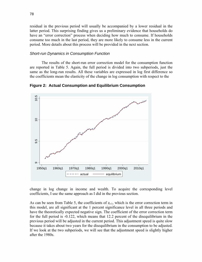
78

residual in the previous period will usually be accompanied by a lower residual in the latter period. This surprising finding gives us a preliminary evidence that households do have an “error correction” process when deciding how much to consume. If households consume too much in the last period, they are more likely to consume less in the current period. More details about this process will be provided in the next section. Short-run Dynamics in Consumption Function

The results of the short-run error correction model for the consumption function are reported in Table 5. Again, the full period is divided into two subperiods, just the same as the long-run results. All these variables are expressed in log first difference so the coefficients mean the elasticity of the change in log consumption with respect to the Figure 2: Actual Consumption and Equilibrium Consumption

99.

510

10.5

1950q1 1960q1 1970q1 1980q1 1990q1 2000q1 2010q1

actual equilibrium

change in log change in income and wealth. To acquire the corresponding level coefficients, I use the same approach as I did in the previous section. As can be seen from Table 5, the coefficients of zt-1, which is the error correction term in this model, are all significant at the 1 percent significance level in all three periods and have the theoretically expected negative sign. The coefficient of the error correction term for the full period is -0.122, which means that 12.2 percent of the disequilibrium in the previous period will be adjusted in the current period. This adjustment speed is quite slow because it takes about two years for the disequilibrium in the consumption to be adjusted. If we look at the two subperiods, we will see that the adjustment speed is slightly higher after the 1980s.

79

Figure 3: The Gap Between Actual and Equilibrium Consumption (Residual)

-.0

4-.

02

0.0

2

1950q1 1960q1 1970q1 1980q1 1990q1 2000q1 2010q1

Residuals

An unexpected finding of this short-run error correction model is that the coefficients of the stock wealth are not statistically significant even at the 10 percent level. This surprising finding is consistent with the results of Case et al. (2005) and Ludvigson and Steindel (1999). According to this result, households will not change their level of consumption in response of the fluctuation in the stock market. However, changes in non-stock wealth like real estate will change the current level of consumption of households. Though the wealth effects of non-stock assets are not very strong – just around a 4 cent increase in the consumption for every one-dollar increase in non-stock wealth – these effects are significant at a 1 percent level. The difference of the wealth effects of stock market in the short run and long run can be explained by the permanent income hypothesis and lifetime-cycle model. Since most of the fluctuations in the total wealth of households are caused by the stock market, households tend to think the fluctuations in their portfolio are transitory and will not change their patterns of consumption significantly in the short run. However, in the long run the accumulated appreciations of their portfolios are stable and households will consider these appreciations as increases in their permanent income. They will correspondingly increase their level of consumption as a result of the increases in their permanent income. Therefore, the stock market wealth does not affect the level of consumption in the short run but have an equilibrium relationship with consumption in the long run.

80

Conclusion and Discussion

This paper reiterates and provides more evidence about the wealth effects of the stock market on the level of consumption. The Koyck model gives a rough estimation about the wealth effects of the stock market. The augmented Dicky-Fuller test indicates that all these variables (consumption, income and wealth) are non-stationary around the trend and are I(1) process. However, the following residual-based cointegration test shows that there is a long-run relationship between consumption, income and wealth. The following dynamic OLS estimates of the consumption function indicate that though stock wealth has significant effects on consumption, the level of marginal propensity to consume out of stock wealth is quite small. For a one-dollar increase in the stock wealth, the level of consumption will only increase by 2 to 3 cents. After dividing the full period into several subperiods, the wealth effects of the stock market vary over time, with a low MPC before the 1980s but a relatively high MPC after the 1980s. These changes in the

Table 5: OLS Estimates of the Short-run Error Correction Model

Estimation period

1

1952Q1-2014Q4

2

1952Q1-1984Q4

3

1985Q1-2014Q4

variable log level log level log level

zt-1

-0.122***

(0.039) -0.122

-0.176***

(0.056) -0.176

-0.203***

(0.069) -0.203

∆in 0.343***

(0.067) 0.385

0.557***

(0.102) 0.624

0.163***

(0.059) 0.183

∆swt -0.001

(0.005) -0.001

-0.0003

(0.007) -0.0004

-0.014

(0.007) -0.017

∆nswt 0.199***

(0.043) 0.039

0.156*

(0.082) 0.030

0.244***

(0.047) 0.047

Notes: the heteroskedasticity and autocorrelation consistent standard errors (HAC) are shown in parentheses. *,** and *** indicate significance at 10 percent, 5 percent and 1 percent level, respectively. wealth effects of the stock market can be explained by the participation rate of household in the stock market. Although the wealth effects of the stock market are very significant in the long run, fluctuation in the stock price will not alter the level of consumption much in the short run. Households might think of fluctuations of stock price in the short run as temporary and will not adjust to them. The coefficients of the error correction terms are also statistically significant and have the theoretically expected sign, which indicates the existence of an adjustment process for the households to recover from the disequilibrium in consumption. However, the value of the coefficients is approximately -0.15 and the adjustment speed is slow. It takes about one and a half years for households to fully adjust from disequilibrium in consumption on average.

81

Though most of the results in this paper are consistent with previous studies, there are still some potential issues in this paper. The first one regards the underlying assumption-“representative agent”. During the analysis of the wealth effects of the stock market in this paper, I assume that a representative agent will hold some amount of equity either directly investing in the stock market or indirectly through mutual funds. In that case, the coefficient in the regression measures the wealth effects of the stock market to everyone in the economy. However, studies have found that actually only part of households in the US hold some wealth in equity form. The participation rate varies dramatically over time and across the wealth level. It has been shown in many studies that the stock market participation rate for the most wealthy people are much higher than that of ordinary people, probably because wealthy people have more assets than ordinary people. For those households who do not hold any stock wealth, the fluctuation in the stock market surely will not affect their level of consumption. Therefore, our estimation of the wealth effects of the stock market actually measures the “average wealth effects” of the stock market. The actual wealth effects of the stock market for those who hold stock wealth should be larger than the average level. However, in order to acquire the wealth effects for the stockholders, we need to divide the population into different parts but the relevant data might be very difficult to find. I believe that further studies, using data for stockholders, can reveal more precise wealth effects for only stockholders, not the whole economy. The second potential issue is about the model specification. By using the error correction model (ECM), we assume that only consumption will change when there is any disequilibrium between consumption, income and wealth. However, we have reasons to believe that income and wealth might also adjust in response to any disequilibrium between them. For example, if one bought a car in the last period, which causes him to overdraft his credit, he might work harder in the current period so that he can earn more and repay the debt in time. In this case, the adjustment will work not only on consumption, but also on income. To incorporate this adjustment, using the vector error correction model (VEC) would be a better choice, which accounts for the adjustment of both income and wealth. The third problem in estimation is about the potential structural changes in the wealth effects. The QLR test indicates that the level of the wealth effects of the stock market are instable over the estimation period. Though this test just shows some preliminary evidences about the instability in the population regression function, we have reasons to believe that the level of the wealth effects are likely to vary over time. Changes in technology, policy and market participation rate will all affect the relationship between the stock market and households’ daily lives and therefore affect how strong the wealth effects are. If these changes happen continuously in the economy, the coefficients of the population regression function will vary smoothly over the estimation period. In this case, our regression estimation of the wealth effects merely tells us what the “average” wealth effects are over that period. To take into account the smooth changes in the parameters, we can use time varying parameter models like rolling regression. We can plot the estimated wealth effects of the stock market against time. If we find that the values of the

82

estimated coefficients vary dramatically over time, we can conclude that the wealth effects are not stable. References Case, Karl E., John M. Quigley, and Robert J. Shiller. (2005). “Comparing Wealth

Effects: The Stock Market Versus the Housing Market.” The B.E. Journal of Macroeconomics 5 (1): 1-32.

Holinski, Nils, and Robert Vermeulen. (2009). "The International Wealth Effect: A

Global Error-Correcting Analysis." Accessed January 16, 2016. http://edocs.ub.unimaas.nl/loader/file.asp?id=1405.

Hong, Harrison, Jeffrey D. Kubik, and Jeremy C. Stein. (2004). “Social Interaction and

Stock-Market Participation”. The Journal of Finance 59 (1). [American Finance Association, Wiley]: 137–63. http://www.jstor.org/stable/3694892.

Ludvigson, Sydney, and Charles Steindel. (1999). "How Important is the Stock Market Effect on Consumption?" Economic Policy Review - Federal Reserve Bank of New York 5, no. 2 (07): 29-51. http://search.proquest.com/docview/210393821?accountid=15115.

Ludwig, Alexander, and Torsten Sløk. (2004). "The Relationship Between Stock Prices,

House Prices and Consumption in OECD Countries." Topics in Macroeconomics 4, no. 1 (Mar 15):1114-1114+. http://search.proquest.com/docview/205531301?accountid=15115.

Macklem, R. Tiff, and Bank of Canada. (1994). Wealth, Disposable Income and

Consumption: Some Evidence for Canada. Vol. no. 71; no. 71.;. Ottawa: Bank of Canada.

Mehra, Yash P. (2001). "The Wealth Effect in Empirical Life-Cycle Aggregate

Consumption Equations." Economic Quarterly - Federal Reserve Bank of Richmond 87, no. 2 (Spring): 45-68. http://search.proquest.com/docview/204890273?accountid=15115.

Pichette, Lise. (2004). "Are Wealth Effects Important for Canada?" Bank of Canada

Review (Spring): 29-35. http://search.proquest.com/docview/230346802?accountid=15115.

Stock, James H., and Mark W. Watson. (1993). “A Simple Estimator of Cointegrating

Vectors in Higher Order Integrated Systems.” Econometrica 61 (4): 783-820. US. Bureau of Economic Analysis (2016). Personal Consumption Expenditures Per

Capita [A794RC0Q052SBEA], retrieved from FRED, Federal Reserve Bank of St. Louis https://research.stlouisfed.org/fred2/series/A794RC0Q052SBEA/, January 14.