2007  

INTERSECTION DATA COLLECTION AND ANALYSIS  GASVERKSVÄGEN – FISKARTORPSVÄGEN  

 

 

 

 

Sam Kaisiromwe

And

Honghu Zhou

  1

 

 

TABLE OF CONTENTS:  Introduction and Background .................................................................2 

Objective ..................................................................................................2 

Data collection description .....................................................................2 

Data Reduction.........................................................................................3 

Gap Acceptance .......................................................................................7 

CAPCAL Results ........................................................................................9 

Round about Results ..............................................................................12 

Discussion ..............................................................................................15 

Recommendations.................................................................................16 

 

  2

 

FISKARTORPSVÄGEN ‐ GASVERKSVÄGEN INTERSECTION 

Introduction and Background 

Traffic volume studies can help agencies make sound traffic safety–related decisions based on data about critical times of traffic flow, the influence of large vehicles or pedestrians on traffic flow, or  trends  in  traffic volume at particular  locations. Traffic volume  studies determine  the number, movements, and classifications of vehicles (and/or bicycles and pedestrians) at specific roadway  locations  at  specific  times.  Some  examples  of  traffic  volume  studies  include  “rush‐hour”  vehicle  counts  at  intersections,  pedestrian  counts,  average  daily  traffic,  and  annual average daily traffic. 

 Fiskartorpsvägen  connects Östermalm  to  Stockholm north,  and  Stockholm University. Under congestion traffic the priority intersection Fiskartorpsvägen ‐ Gasverksvägen is oversaturated.   

Objective  The objective of the project  is to collect data about the actual situation, analyze them and to suggest design changes to improve safety and performance.  Methodology The  computer  programme  CAPCAL was  chosen  as  the  tool  for  analyzing  and  evaluating  the performance  of  the  intersection. Other Geometry  data  and  input  speeds  and  relevant  data were collect from the field using data logger and video. The video was analyzed in the lab to get vehicle counts and turning movements. 

Data collection description  

Automatic  data  collection  methods  were  used  at  the  junction  to  collect  data.  Automatic counting methods are used to gather large amounts of traffic data over an extended period of time. Counts are generally collected for 1‐hour intervals in 24‐hour periods. Automatic counting methods are generally used to determine traffic patterns and trends. The following information can be determined using automatic counts: 

• hourly traffic patterns  • daily or seasonal variations  • growth trends  • annual traffic estimates  

Observers can use portable or permanent automatic counters  in this data collection exercise, portable counters were used. Portable counters consist of automatic  recorders connected  to pneumatic road tubes. These tubes were connected to an automatic traffic data logger and set to collect data for the specified period. They are typically used to collect the same kind of data collected  in manual counts, but  for  longer periods, usually 24 hours. Permanent counters are 

sometimes built into the pavement and used for long‐term counts. The equipment is expensive, and relatively few  jurisdictions have access to  it. With this method, data on speeds, time, and flow of vehicles can be measured 

Video  data  collection method  at  the  junction was  also  used,  the  turning  count  information, registration number plate  identification collected as part of this study was derived from video analysis, where  the  cameras  are mounted  so  as  to  capture  all  the  entries  and  exits  to  that specified  junction over a  specified period.   These videos were  then analyzed manually  in  the computer lab and the results summarized by time and vehicle types with API programme. 

 

Data Reduction 

 

 

Fig.  1  shows  the  position  of  the  junction  and turning traffic. 

Using  the  overhead  video  recordings  on DVD, all the points 1, 2…., 6 were viewed and  vehicles passing  them  for every  five (5) minutes were  counted and  recorded as below. 

The  results  show  that  the  through vehicles  from  K1  to  K2  flow  least  at  48 vehicles per hour and stream 1 (turn right from  K1)  had  the  highest  flow  of  306 

vehicles  per  hour.  The  rest  of  the  turns registered  a  flow  that was below  200  vehicles 

per hour. See table 1 below. 

  

 

Tab: 1 Number of vehicles passing  at each stream point every after 5 minutes point  TIME  TOTAL FLOW 

  12:30‐‐12:35 

12:35‐‐12:40 

12:40‐‐12:45

12:45‐‐12:50  (20 MIN.)  V/HR

1  29  32  21 20  102  3062  4  3  6 3  16  483  9  2  2 6  19  574  16  20  13 17  66  1985  16  12  13 23  64  1926  30  17  28 23  98  294

 

 

 

 

 

 

  3

Fig 2. Relationship between Flow and Speed  

 

 

Tab: 2 Channel Pair: 2 ‐ 3 Total Report Period: 12:30 to 13:30 

      K1 K2 K1  K2 

 Total vehicle identified     705 436 Proportion  Proportion 

 Car               608                368                         0.86           0.84  

 Lorry/Bus                27                  21                         0.04           0.05   Van/Mpv                19                  11                         0.03           0.03  

 Cycle                41                  29                         0.06           0.07  

 MC                 10                    7                         0.01           0.02   

The table above shows the proportion of vehicles passing at point K1and K2 of the junction. It was observed that 86 percent of the vehicles passing point K1 were passenger cars, 6.0 percent are motorcycles. Vans and lorries/buses were 3 and 4 percent respectively. The rest 1.4 percent were MCs  and  it was  noted  that  no  Semis were  observed  at  that  point.  At  K2  84  percent vehicles  registered were passenger  cars and  the  rest  shared 16 percent as  shown  in  table 2 above.  

 

 

 

  4

  5

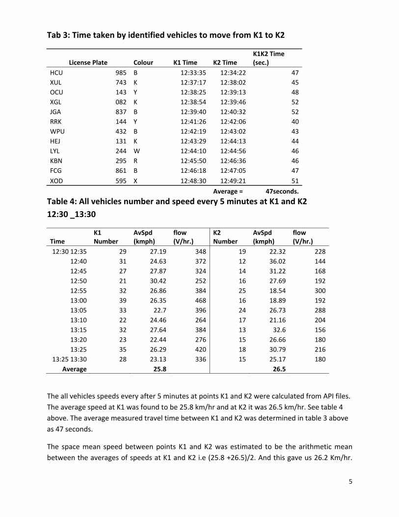
Tab 3: Time taken by identified vehicles to move from K1 to K2 

License Plate  Colour  K1 Time  K2 Time K1K2 Time (sec.) 

HCU  985  B  12:33:35 12:34:22 47 XUL  743  K  12:37:17 12:38:02 45 OCU  143  Y  12:38:25 12:39:13 48 XGL  082  K  12:38:54 12:39:46 52 JGA  837  B  12:39:40 12:40:32 52 RRK  144  Y  12:41:26 12:42:06 40 WPU  432  B  12:42:19 12:43:02 43 HEJ  131  K  12:43:29 12:44:13 44 LYL  244  W  12:44:10 12:44:56 46 KBN  295  R  12:45:50 12:46:36 46 FCG  861  B  12:46:18 12:47:05 47 

XOD  595  X  12:48:30 12:49:21 51 

        Average =  47seconds. 

Table 4: All vehicles number and speed every 5 minutes at K1 and K2                                             12:30 _13:30 

Time K1 Number 

AvSpd  (kmph) 

flow (V/hr.) 

K2 Number 

AvSpd (kmph) 

flow (V/hr.) 

12:30 12:35  29  27.19 348 19 22.32  22812:40  31  24.63 372 12 36.02  14412:45  27  27.87 324 14 31.22  16812:50  21  30.42 252 16 27.69  19212:55  32  26.86 384 25 18.54  30013:00  39  26.35 468 16 18.89  19213:05  33  22.7 396 24 26.73  28813:10  22  24.46 264 17 21.16  20413:15  32  27.64 384 13 32.6  15613:20  23  22.44 276 15 26.66  18013:25  35  26.29 420 18 30.79  216

13:25 13:30  28  23.13 336 15 25.17  180Average    25.8 26.5 

 

The all vehicles speeds every after 5 minutes at points K1 and K2 were calculated from API files. The average speed at K1 was found to be 25.8 km/hr and at K2 it was 26.5 km/hr. See table 4 above. The average measured travel time between K1 and K2 was determined in table 3 above as 47 seconds. 

The  space mean  speed between points K1 and K2 was estimated  to be  the arithmetic mean between the averages of speeds at K1 and K2  i.e (25.8 +26.5)/2. And this gave us 26.2 Km/hr. 

  6

Average delay between K1 and K2 is obtained by getting the time taken to move between the points at space mean speed, then we subtract the actual average measured time of 47 seconds. 

• Space Mean Speed = 26.2 km/hr 

• Distance between K1 and K2 = 171 m = 0.171km 

• Time = Distance/speed    = 0.171/26.2     0.006527 hrs.     23.5 seconds. Therefore the delay is given by 47 – 23.5 = 23.5 seconds. 

 

Tab 5: Determination of average delay for the K3 Lane 

Point of time  Number of     Point of time  Number of 

for observation i Vehicles in queue     for observation i 

Vehicles in queue 

12:30:00  0   12:41:30 5 12:30:30  3   12:42:00 0 12:31:00  2   12:42:30 0 12:31:30  3   12:43:00 0 12:32:00  0   12:43:30 0 12:32:30  0   12:44:00 0 

12:33:00  0   12:44:30 2 12:33:30  1   12:45:00 0 12:34:00  4   12:45:30 0 12:34:30  0   12:46:00 8 12:35:00  0   12:46:30 3 12:35:30  0   12:47:00 1 12:36:00  0   12:47:30 6 12:36:30  0   12:48:00 0 12:37:00  0   12:48:30 0 12:37:30  0   12:49:00 5 12:38:00  0   12:49:30 8 12:38:30  0   12:50:00 0 12:39:00  0      

12:39:30  4      12:40:00  0        12:40:30  0   Sum N  55 12:41:00  0         

  Total number of vehicles that were in queue after 20 minutes were 55 Total number of vehicles that had passed the point after 20 minutes were 162 

  7

               Using the formula, d = ⅟Q ∑Ni * 30             

 55x30/162             =10.2  Seconds             

Where,  

D = average delay  

Q = number of departed vehicles in the lane during the studied period 

Ni = Number of queuing vehicles at observation i 

Note: Delay obtained by  the group  that used SAVA  to determine  the difference between  the 

real travel time and cruise time was about 9seconds. 

Gap Acceptance 

Introduction Gap  acceptance  is  an  essential  skill  for  safe  driving.  Road  crossing  is  a  complex  perceptual‐motor task that requires accurate perception of the gap sizes in a dynamic stream of traffic and fine  coordination  to  synchronize  the  onset  of  movement  with  the  approaching  gap. Understanding how drivers decide that a gap  is crossable and how they time their crossing  in relation to a moving stream of traffic is critical for the development of training and technology to lower the risk of crashes.   Definitions  In  this study, a gap  is defined as  the  time elapsed between  the successive passage of major‐road vehicles as measured from a given reference line. A lag is the time between the departure of a minor‐road vehicle and the arrival of the next major‐road vehicle at a given reference line. The  departure  time  is  defined  as  the  time when  the  vehicle  either  arrives  at  or  leaves  the minor‐road reference line.   

Data needed 

The  collection  of  quantitative  gap  data  is  the  first  step  for  any  gap  acceptance  study.  The arrivals of vehicles on the major road, and the arrivals and departures of vehicles on the minor road are among the most basic data that need to be collected. In order to capture the arrival of major‐road  vehicles,  a major‐‐  road  reference  line  is  usually  used. Many  practices  exist  for recording  the  arrival  and  departure  of minor‐‐  road  vehicles.  But  in  this  project,  data was collected automatically according at the stop/yield line, using data logger connected to buttons which  observers were  punching  as  the  vehicle  reaches  and  leaves  the  stop  line.  The  same vehicle would then be monitored until it reaches point C at K2. 

  8

 

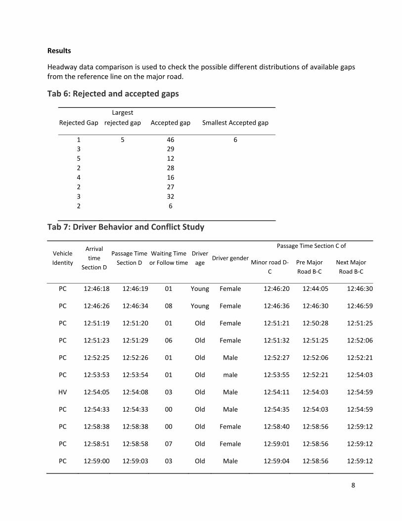
Results 

Headway data comparison is used to check the possible different distributions of available gaps from the reference line on the major road.  

Tab 6: Rejected and accepted gaps 

Rejected Gap Largest 

rejected gap  Accepted gap  Smallest Accepted gap 

1  5  46  6 3    29   5    12   2    28   4    16   2    27   3    32   2     6           

Tab 7: Driver Behavior and Conflict Study 

Passage Time Section C of Vehicle Identity 

Arrival time 

Section D 

Passage Time Section D 

Waiting Time or Follow time

Driver age 

Driver genderMinor road D‐

C Pre Major Road B‐C 

Next Major Road B‐C 

PC  12:46:18  12:46:19  01  Young Female  12:46:20  12:44:05 12:46:30

PC  12:46:26  12:46:34  08  Young Female  12:46:36  12:46:30 12:46:59

PC  12:51:19  12:51:20  01  Old  Female  12:51:21  12:50:28 12:51:25

PC  12:51:23  12:51:29  06  Old  Female  12:51:32  12:51:25 12:52:06

PC  12:52:25  12:52:26  01  Old  Male  12:52:27  12:52:06 12:52:21

PC  12:53:53  12:53:54  01  Old  male  12:53:55  12:52:21 12:54:03

HV  12:54:05  12:54:08  03  Old  Male  12:54:11  12:54:03 12:54:59

PC  12:54:33  12:54:33  00  Old  Male  12:54:35  12:54:03 12:54:59

PC  12:58:38  12:58:38  00  Old  Female  12:58:40  12:58:56 12:59:12

PC  12:58:51  12:58:58  07  Old  Female  12:59:01  12:58:56 12:59:12

PC  12:59:00  12:59:03  03  Old  Male  12:59:04  12:58:56 12:59:12

  9

 

CAPCAL Results  

The performance of  traffic operations at an  intersection can be  represented by  the  following measures of effectiveness:   

• Degree of saturation (volume/capacity)  • Average delay  • Average queue length • Distribution of delays  • Distribution of queue lengths (i.e. number of vehicles queuing on the minor road)  • Number of stopped vehicles  

Of recent, environmental costs and operational costs at the junction have emerged to play a big role in any traffic and transport data analysis and evaluation.  In addition to operational data, a variety of geometric data have been extracted from the plans. The geometric data are principally various distance measurements, radii, and angles that affect the way in which vehicles traverse the roundabout. Some of the data items can be read directly from the drawings, while others have to be derived from paths or trajectories that are traced through the roundabout based on the manner in which an experienced design engineer thinks the vehicles will travel from entry points to exit points. 

Tab 8: Geometry Data. Geometry       

Approach  Radius RT  Angle  Gradient (%)

A  24  120  0 

B  8  60  0 

D  5  90  0 

We  assumed  that  the median  length  for  all  lanes was  5 m  and  vehicles were  approaching intersection at a speed of 50 km/hr.  A 10 % of heavy vehicles correction was also applied. The results were as below. 

 

 

 

 

 

 

  10

Tab 9: Capacity and degree of saturation per lane 

  Lane  Movement Volume (vph) 

Capacity (vph) 

Degree of saturation

Queue length mean   

A  1  RL  460  821  0.56  1   

B  1  RT  450  1818  0.25  0   

D  1  T  190  1668  0.11  0   

  2  L  60  722  0.08  0.1   

                       

 

Tab 10: Delay and number of stops per lane 

        Percent delayed     

Approach  Lane Delay spv Conflict 

Geometric delay. 

Total delay  Conflict  Stops 

Geometric delayed  Total 

A  1  8  5  10  63  23  37  100 

B  1  0  4  4  0  0  89  89 

D  1  0  0  0  0  0  0  0 

  2  3  6  6  48  15  52  100 

All vehicles  3  4  6  28  10  52  79 

 

Tab 11: Annual Average Daily Traffic AADT 

  Axle pairs  Private cars  Heavy vehicles 

Heavy vehicles 

with trauler Total 

A  5668  4669  259  259  5188 

B  5855  4823  268  268  5359 

D  2927  2412  134  134  2680 

Total  14451  11904  661  661  13227 

 

The  first output at the  junction gave the  following results; degree of saturation of  lanes A, B, and D were 0.56, 0.25, and 0.11 respectively. Queues were only observed on  lane A with the 

  11

queue mean  length of 1. The  total delay per  lane was 10, 4 seconds  for approaches A and B respectively. Approach D  lane  1 did not  register  any delay  after  the CAPCAL  runs.  The  total delay of the  junction for all vehicles was recorded as 6 seconds. For more details see tables 9 and 10 above 

It should be noted that, as vehicles are delayed, stopped at any junction, they tend to use more fuel  and  experience  tyre  worn  outs,  thus  a  capital  cost  to  the  owners.  However  as  they consume more  fuel,  they  emit  dangerous  gases  such  as  corbondioxide,  nitrogen  oxide  and others.  These  gases  are  a  problem  to  the  environment  and  therefore  to  people  around  the junction. A value is always attached to such externalities in order to measure the extent of their destruction. The table below shows the valued problems that are associated with the junction. 

 Tab 12: Total Costs per year of the intersection. 

  Private cars 

Heavy vehicles 

Heavy vehicles with trailer  Total 

Fuel costs  107454 12116 61427 180997

Vehicle costs         

  Capital  48110 36907 104536 189553

  Tyre  4854 6720 10189 21764

Total vehicle cost  52964 43627 114726 211317

Environmental costs         

  NOX  7561 10715 64396 82672

  SO2  12 2 10 24

  VOC  5331 ‐215 350 5466

  Particles  0 0 0 0

  CO2  153119 24555 124488 302162

Total  166024 35057 189244 390324

Time costs         

  Value of time  780607 78717 78717 938040

  Value of goods  0 3644 18221 21866

Total  780607 82361 96938 959906

Total  1107048 173161 462335 1742544

  Accident costs           710737

Total incl. accident costs           2453281

 

Round about Results 

Roundabouts  represent  a unique  blending  of  operations, safety,  and  design,  where changes to one element appear to  have  a  significant  effect  on the  others.  A  roundabout intersection  brings  together conflicting  traffic  streams, allows  the  streams  to  safely merge  and  transverse  the roundabout,  and  exit  to  their 

desired direction. Drivers approaching a roundabout must slow to a speed that will allow them to safely  interact with other users, and to negotiate the roundabout. As drivers approach the yield  line,  they must  check  for  conflicting  vehicles  already  on  the  circulating  roadway,  and determine when it is safe to enter the one‐way circulating stream.    

Some definitions 

 

Three performance measures are typically used to estimate the operational performance of a roundabout: degree of  saturation, delay  and queue  length. Each measure provides  a unique 

  12

  13

perspective on the quality of service at which a roundabout will perform under a given set of traffic and geometric conditions 

 

 

Tab 13: Capacity and degree of saturation per lane 

  Lane  Movement Volume (vph) 

Capacity (vph) 

Degree of saturation

Queue length mean   

A  1  RL  460 1421 0.32 0  

B  1  RT  450 1426 0.32 0  

D  1  T  190 1098 0.17 0  

  2  L  60 1046 0.06 0  

        

 

Tab 14: Delay and number of stops per lane 

        Percent delayed    

Approach  Lane Delay spv Conflict 

Geometric delay. 

Total delay  Conflict  Stops 

Geometric delayed  Total 

A  1  0  5 3 15 0 85  100

B  1  0  4 3 14 0 86  100

D  1  1  7 4 38 1 62  100

  2  1  9 3 35 0 65  100

All vehicles    0 5 3 20 0  80

 

 

 

 

  14

Tab 15: Total Costs per year for the round about. 

  Private cars 

Heavy vehicles 

Heavy vehicles with trailer  Total 

Fuel costs  84410 10286 55093 149790

Vehicle costs         

  Capital  44396 31331 90057 165784

  Tyre  2825 3912 5931 12668

Total vehicle cost  47221 35243 95988 178452

Environmental costs         

  NOX  7148 9371 58054 74573

  SO2  9 2 9 20

  VOC  4759 ‐440 332 4652

  Particles  0 0 0 0

  CO2  120283 20846 111652 252781

Total  132200 29779 170046 332026

Time costs         

  Value of time  454365 45818 45818 546001

  Value of goods  0 2121 10606 12727

Total  454365 47939 56424 558728

Total  718196 123248 377552 1218996

  Accident costs        382850

Total incl. accident costs        1601846

 

 

 

 

 

 

 

 

 

  15

Discussion  

Summary of the results for the junction and roundabout 

In this summary we shall  look at the main  indicators of performance  in both scenarios, these are Delay, Queue length, Degree of saturation and externalities costs. 

Tab 16: Comparison between the Intersection and Roundabout. 

       Intersection Roundabout %change 

                 1  Queue length           A  1 0      B  0 0      D  0 0             

2  Total Delay  6 5 17     A  10 3 70     B  4 3 25     D  6 4 33            3  Degree of saturation           A  0.56 0.32      B  0.25 0.32      D  0.11 0.17             4  Total Costs           Vehicle & fuel costs  392,314 328,242 16.3     Environmental costs  390,324 332,026 14.9     Time costs  959,906 558,728 41.8 

     Accident costs  710,737 382,85 46.1       TOTAL  2,453,281 1,601,846 34.7 

 

The queue  length was  identified on the arm A (K3) of the junction with a  length of 1, this was reduced  to  zero  after  the  roundabout  implementation.    Total  delay  for  the whole  junction reduced from 6 minutes to 5 minutes after the implementation of the roundabout. This was a 17  percent  reduction  in  delay.  The  arm  A  delay was mostly  reduced  from  10  seconds  to  3 seconds, a 70 percent reduction. Arm D of the intersection had a total delay of 6 seconds that were  later  reduced  to  4  seconds  after  the  roundabout  implementation  this  reflected  a  33 percent reduction.  

  16

Degree of saturation is defined as the ratio of flow to the capacity of the road. It is known that the less the value of degree of saturation the better the road in study.  On average the degree of saturation reduced  from 0.30 at the  intersection to 0.27  for the roundabout, showing that the capacity of the intersection increased with a change to roundabout. 

The total costs at the roundabout reduced from 2,453,281 at the intersection to 1,601,846 for the roundabout, a reduction of 34.7 percent. Accident costs per year reduced by 46.1 percent after implementing the roundabout. 

 

Recommendations 

We recommend that the intersection be redesigned into a round about because the queue will disappear  and  the  delay  at  the  junction will  reduce.  Also  the maintenance  costs  to  vehicle owners will reduce and we noted that the environmental effects will improve. 

 

Limitations: 

Because of the nature of data collection from the field, the input data into the API files may not be accurate due to the following reasons 

• The difference between observing  and pressing of buttons (response time and pressing error) for different data collectors 

• Topography of  the area which especially  from  the K3 arm  that did not  give drivers a good clearing distance to the intersection. 

• Only vehicle traffic is analyzed, pedestrians and cyclists are ignored 

• The study period is too short to make any sound conclusions. 

 

References 

• Transport Planning and Traffic Engineering By C A O’Flaherty 

• Improvement  of  Traffic  Performance  and  safety  of  four  intersections  on Kringlumy’rarbraut in Reykjavik(Master’s Thesis) By SGRUN MARTEINSDOTTIR