Are Consumers Averse to Sponsored Messages? The Role of Search

Advertising in Information Discovery*

Navdeep S. Sahni

Stanford GSB

Charles Zhang

Stanford GSB

October 2020�

Abstract

We analyze a large-scale randomized field experiment in which a search engine varied the prominence of

search ads for 3.3 million US users: one group of users saw the status quo, while the other saw a lower level of

advertising (with prominence of search ads decreased). Revealed preference data reject that users are, overall,

averse to search advertising targeted to them across a diverse set of searches. At the margin, users prefer

the search engine with the higher level of advertising. On the supply side, newer websites are more likely to

advertise. Going from the lower to the higher level of advertising increases traffic to newer websites, with the

newest decile of websites gaining traffic by 10%. Users also respond more positively to advertising when local

businesses in their state create new websites.

Taken together, patterns in our data are consistent with an equilibrium in which advertising compensates for

important information gaps in organic listings: it conveys relevant new information, which is hard for the search

engine to gather, and therefore missed by the organic listings algorithm. Viewing search ads, at the margin we

study, makes consumers better off on average.

*The views discussed here represent that of the authors and not of Stanford University. We are thankful for comments from Pe-dro Gardete, Gagan Goel, Sachin Gupta, Wes Hartmann, Carl Mela, Sridhar Moorthy, Harikesh Nair, Sridhar Narayanan, DeveshRaval, Stephan Seiler, Andrey Simonov, Raluca Ursu, Caio Waisman, and from participants at the AFE Conference University ofChicago, MIT Conference on Digital Experimentation, CMU Digital Marketing and ML conference, 2019 Choice Symposium, 2019& 2020 Marketing Science conference, Marketplaces and Algorithms Design seminar 2020; seminars at Yale SOM, Google, Washing-ton Univ, Harvard Business School, SMU, Univ of Florida, Santa Clara Univ. The usual disclaimer applies. Please contact Sahni(navdeep.sahni@stanford.edu) or Zhang (cyzhang@stanford.edu) for correspondence.

�Previous drafts: Aug 23 2019; October 2019; June 2020.

1

1 Introduction

Researchers have long theorized about the effects of advertising and have arrived at differing views on its role in a

market. Some have proposed that advertising plays a constructive role by enabling firms to convey economically

relevant information to consumers, thereby improving market efficiency (e.g., Stigler 1961; Telser 1964). Others

(e.g., Robinson 1933; Kaldor 1950; Galbraith 1967) have been skeptical about the relevance of the actual information

consumers get from seeing the ads supplied to them, and construe advertising as overall anti-competitive.1 Under

this view, as Bagwell (2007, p. 1705) summarizes, “[advertising] has no ’real’ value to consumers, but rather induces

artificial product differentiation and results in concentrated markets characterized by high prices and profits.”

Theory alone cannot determine the actual role of advertising. It depends on whether consumers are sophisticated

enough to recognize and demand for relevant advertising, and whether the media market is incentivized to supply

it to the consumers. These conditions are not guaranteed by theory.2

In this paper, we take an empirical approach to assess the value consumers get from seeing ads supplied by digital

markets, and ask: can the market mechanisms supply ads that provide a positive value to consumers, overall?3

Empirically assessing the overall utility consumers get from viewing an ad is challenging, in general, primarily

because of the following two reasons. Firstly, viewing an ad can simultaneously provide utility and disutility in

different ways. While some consumers may get positive utility from the information contained in the ad, others

may get disutility from the presence of advertising if it leads them to make suboptimal decisions (e.g., by diverting

their attention away from their best-suited product). Additionally, all consumers exposed to the ad incur time

costs when they view it. Measuring all these effects is difficult. Secondly, data on the right counterfactual – a

change in the overall level of advertising – is hard to observe. To assess the value of advertising consumers get

exposed to, one needs to observe outcomes in a counterfactual scenario where consumers do not get exposed to

advertising they would have seen, holding everything else the same. Data on such scenarios are rare.

These challenges make it difficult to learn about the utility consumers get from viewing ads using approaches

common in the prior research. One approach is to estimate this value by examining the effect of advertising on

purchase of the advertised product and its category (see e.g., Ackerberg 2001; Tellis, Chandy, and Thaivanich 2000;

Erdem, Keane, and Sun 2008; Mehta, Chen, and Narasimhan 2008; Clark, Doraszelski, Draganska, et al. 2009).

This approach is able to show the value of advertising derived by a subset of consumers – usually a small fraction

1For example, Kaldor (1950, p. 5) says “As a means of supplying information, it may be argued that advertising is largely biassedand deficient ... the information supplied in advertisements is generally biassed, in that it concentrates on particular features to theexclusion of others; makes no mention of alternative sources of supply; and it attempts to influence the behaviour of the consumer, notso much by enabling him to plan more intelligently through giving more information, but by forcing a small amount of informationthrough its sheer prominence to the foreground of consciousness.”

2The theory literature on persuasion (see e.g., Milgrom 2008) shows that, while persuasive communication may manipulate naıveconsumers, consumers that are rational and skeptical about the information they receive will push senders to provide useful informationin equilibrium. Summarizing the economic forces governing usefulness of persuasive messages, DellaVigna and Gentzkow (2010, p. 658)note: “A countervailing force for accuracy [of persuasive messages] is the desire to build a reputation: If receivers are rational, sendersmay benefit from committing to limit the incentive to distort, or to report accurately. These two forces—the incentive to distort andthe incentive to establish credibility— play out differently in different markets, and their relative strength will be a key determinant ofthe extent to which persuasive communications have beneficial or harmful effects.”

3The value consumers get from seeing ads at the margin, which we empirically study, is particularly unclear because ads are oftenrepetitive. Furthermore, there is a multitude of other information such as product reviews available to consumers on the internet sothe value consumers get from digital ads might be low.

2

of total ad viewers – who change their decision of buying the advertised product because of advertising. However,

this approach does not account for utility / disutility advertising may cause through other avenues, for example,

the cost of time spent viewing the ad, incurred by all consumers who saw the ad. Further, most studies compare

the effect of one advertiser’s ad relative to a counterfactual scenario that replaces that ad with a different one.

Hence, a decrease in the overall level of advertising (which comprises of a representative set of advertisers) is not

observed.

An alternative approach is to survey individuals and use stated preference data to assess the value of viewing ads

(see e.g., Finn 1988; Singh, Rothschild, and Churchill Jr 1988; Malhotra et al. 2006 for an overview). A primary

challenge with this approach arises due to low reliability of stated preferences, which may be distorted by errors in

recall (Roediger and McDermott 2000), and potential inaccuracy in a consumer’s overall assessment of the value

of past advertising (see e.g., Aribarg, Pieters, and Wedel 2010).

Finally, a third approach is to focus on the content of ads, and document the presence / absence of potentially

valuable information such as price and product attributes (e.g., Resnik and Stern 1977; Abernethy and Franke 1996;

Anderson, Ciliberto, and Liaukonyte 2013). Since this approach does not take into account consumers’ assessment

of the ads, employing it to estimate the extent of the usefulness of ads to consumers who actually see them is hard.

Further, since the total information consumers are exposed to in the presence and absence of ads is unobserved,

using this approach to assess even the direction of the effect of advertising on consumer information is challenging.

We overcome the above challenges by using unique revealed preference data from a large-scale field experiment in

the context of internet search in the US. We use the experiment, which spans 3,298,086 consumers and a diverse set

of 147,273 advertisers, to investigate whether viewing more search advertising provides overall positive or negative

utility to consumers. Internet search is an important context to study because it is a primary means of information

gathering, in general.4 Consumers often begin their searches on search engines that are mainly financed by search

advertising, which is one of the largest categories of advertising media (accounting for 19.8% of total ad spending

in the US in 2018 eMarketer 2019).

The experiment, detailed in section 4, was run on a widely-used search engine (our data provider) that selected a set

of users and randomized them into a treatment and a control group. For a period of two months the control group

users experienced, on average, a reduced prominence of search advertising on any search they conducted during

this time period. The prominence of advertising on a page was reduced by removing marginal search ads from the

center of the page (also known as the “mainline”) and moving them to the column on the page’s right-hand-side.

In expectation, this change reduces the number of ads (and increases the number of organic listings) control group

users see on any search-results page. There is no such change for the treatment group, which experiences the status

quo. We refer to this group as the treatment group because we are interested in the effect of advertising and this

group is expected to be “treated” with more ads; in expectation this group sees a higher number of ads (and a

4An estimated 16 billion search queries were conducted from US desktop computers in October 2018, with two-thirds of these searchqueries being handled by Google and most of the remaining queries being handled by Microsoft’s Bing and Oath’s Yahoo (Comscore2018). Among other things, consumers often search for information about current events (e.g., news, sports, celebrities), professionaladvice (e.g., medical, financial, legal) and products (reviews, price comparisons, new products). Examples of the variety of informationsought by users can be seen at https://trends.google.com/trends/yis/2018/US/. Another common type of information often sought byconsumers is the location (URL) of a specific website or online service.

3

lower number of organic listings) relative to the control group. All other aspects of the search experience (including

the identity of the advertisers and the organic listings) are held constant.5

This experiment design simulates two counterfactual worlds in which only the prominence of advertising, and

therefore, the expected number of ads seen is changed. In the data we observe several aspects of the information

consumers get exposed to, as well as consumers’ usage of the search engine during, before, and after the experiment,

which allows us to assess how consumers respond to our treatment. If viewing ads creates disutility and imposes

a “cost” on the consumer, we expect consumers in the treatment group – who are exposed to more prominent

advertising – to reduce their search engine usage relative to the control group both during and after the experiment.

If utility from seeing ads is positive and greater than the utility from seeing the marginal organic listings, higher

prominence of advertising would be preferred and we expect to see the opposite pattern.

Furthermore, the availability of detailed data allows us to empirically support our inference and examine alternative

explanations. Using historical data we compare the treatment effect on users who are likely to have lower switching

costs, with the treatment effect on other users to support our inference that the treatment effects measure changes

in demand for the search engine. In sum, our approach overcomes the empirical challenges in answering our question

by using experimental randomization, and focusing directly on demand for advertising, as opposed to demand for

the products being advertised.

Results Analyzing our experiment, we first assess the effect of the treatment on information seen by the search

engine users. We find that going from control to treatment (making search advertising more prominent) increases

the number of search ads presented in the mainline by 20%. Analyzing the actual content presented to users, we

find that the experimental treatment causes placement of more unique websites, newer and more popular websites

in the center of users’ screens.6 This suggests that, on average, the marginal ad in our experiment adds unique

information, and does not merely repeat websites that are already present in the organic listing.

Our experimental treatment affects user clicking behavior. From control to treatment group ad clicks increase by

4.20% and organic clicks decrease by .78%. Overall, search engine revenue increases by 4.3-14.6% in our estimation.

Notably, we find no evidence of consumers decreasing their usage of the search engine when advertising is increased.

On average, the number of searches by users after the experiment begins is higher in the treatment group relative

to those in the control group (who see less prominent advertising) by 2.47%. Treatment group users also engage in

more search sessions, which is a key metric used by search engines to track user experience (see e.g., Kohavi et al.

2012).7 Our estimation of quantile treatment effects shows that the experimental increase in the prominence of

search ads shifted the distribution of the number of searches, and the number of sessions upwards (i.e., increased

the number of searches, and the number of sessions). This pattern persists even after the experimental period when

the experimental variation ends.

5Since our experiment affected a small proportion of the search engine’s user base, we assume aspects such as advertiser behaviorwere not affected by our experiment. Hence, our design enables the assessment of ads in the context in which they naturally appear.

6We assess newness and popularity of websites by using Comscore web panel dataset, as detailed in section 5.7A session is a collection of the user’s searches. A new session is initiated whenever a user conducts a new search that takes place

more than 30 minutes after the last search they conducted on the search engine. Kohavi et al. (2012) discuss Bing search engine’s“overall evaluation criteria” (OEC) and mention that the number of sessions per user is a key component of it.

4

Consumers with lower cost of switching to a competing search engine are likely to be more sensitive to changes

in the search engine’s usefulness relative to the average consumers. Hence, if higher prominence of advertising

is undesirable we expect these likely switchers to respond more negatively to the experimental treatment. To

investigate this, we analyze users who we observed searching for a competing search engine prior to the experiment.

We find that these users significantly increase their usage of the search engine because of an increased prominence

of advertising, and this increase is larger than that for average users.

Additional Supporting Analysis We find that consumer benefit from advertising increases when (a) ads are

more relevant and (b) organic listings are less relevant. We find that the change in usage caused by our experimental

treatment is positively correlated with a change in clicks on the ads, which is a proxy for the ad being relevant

to the consumer. Further, the effect on search engine usage appears with a lag: while the experiment causes an

immediate increase in ad clicks, the increase in searches occurs at least a day after the increase in ad clicks. In

addition, we find that our treatment effect is higher in instances where the consumer enters a search query for which

the organic listings have had low historical click-through rates, or organic listings are repetitive, that is, linked to

the same website. These are both situations in which the marginal organic listings are likely to be less informative

and, consequently, making ads prominent may be beneficial.

Interpretation and Underlying Mechanism Our interpretation of these results is that, in our context, the

search engine market is able to supply the consumer with useful information in the form of advertising. Seeing the

marginal ad increases a consumer’s future expectation of finding useful information on the search engine. Therefore,

consumers are more likely to return to the search engine and use it more in the future. Overall, users prefer the

search engine when it shows advertising more prominently.

Next, we investigate deeper to explain our findings. We consider a mechanism in which some firms have private

information – unknown to the search engine – which increases the consumer’s demand for the advertiser when

revealed to them. In equilibrium, the search engine sorts firms by its assessment of relevance to the consumer’s search

query and places them in the organic listing, without accounting for the firm’s private information. Advertising

enables firms to convey their private information. Firms with most impactful private information advertise to

convey it, in equilibrium. A stylized model in Appendix A explains our mechanism more precisely.8

We empirically examine the presence of this mechanism. Based on our review of the published discussions on search

engine algorithms (detailed in 3.1), we presume that new websites are most likely to have consumer-search-relevant

private information. A search engine’s assessment of a website depends partially on the number of other websites

referring to it, and the quality of the referrers. Therefore, by design, a new website is at a disadvantage when being

assessed by the search engine: it gets underplaced in the organic listings because getting recognized and cited by

other websites takes time.

8This mechanism is consistent with the classical view that individual businesses possess valuable contextual information that centralorganizations do not have (Hayek 1945). It is also consistent with a signaling role of search advertising (Nelson 1974; Sahni and Nair2018).

5

Our mechanism predicts that advertising provides a way for new websites to reach relevant users. To check for

this in our data, for each website, we estimate the difference between the clicks (ads + organic) received from

our experimental treatment and control group users. We find that this difference is largest for newest websites, in

both relative and absolute terms, suggesting that the experimental increase in prominence of advertising is most

beneficial to new websites in terms of immediate traffic they receive. This finding is robust to controlling for the

website’s popularity, and repeat usage.

Our mechanism also predicts that a user’s benefit from advertising increases with the presence of websites that are

relevant to their search need but missed by the organic algorithm. To check this prediction, we use variation in the

internet presence of local businesses across the 50 states in the US, and over time.9 Specifically, we use data from

US Census Bureau’s 2016 Annual Survey of Entrepreneurs (ASE), which measures the number of local businesses

within a state that have their own website. Based on this measure, we categorize states into four quartiles. Merging

this data with our main analysis dataset we find that the effect of advertising on search engine usage is highest

in states where the highest proportion of local businesses have websites. Further, our experimental treatment

increases search engine usage more in states where more businesses have created websites within the previous two

years (between 2014, the first year of ASE, and 2016). This finding persists even after we control for change in

GDP between 2014 and 2016, and per capita income of the state. These data patterns suggest that advertising is

more helpful to consumers when more local businesses have an internet presence, and more so when their websites

are relatively new.

Overall, our data indicate advertising can serve as an instrument to help uncover useful information that aggregators

such as search engines systematically miss, despite processing vast amount of data. This differs from an alternative

view that having to see ads is merely a “price” users pay for free access to the search engine – users are drawn to

the search engine solely due to organic listings, and the search engine bundles organic results with search ads to

increase its payoff (e.g., Rayo and Segal 2010). By this alternative view search engines would compete by reducing

advertising. On the other hand, our mechanism suggests search engines would compete by enabling mechanisms

that improve the quality of their advertising; removing ads completely might make the search engine less appealing

to its users.

By providing evidence of consumers getting an overall positive utility from search ads, this paper complements a

large theoretical literature that conceives of advertising as informative about a product’s existence and its attributes

(Stigler 1961; Butters 1977), or increasing consumer’s utility of the product (Stigler and Becker 1977), or serving

as a signal for product quality (Nelson 1974; Milgrom and Roberts 1986; Kihlstrom and Riordan 1984). Consistent

with the mechanism in Grossman and Shapiro (1984), we show that search advertising increases awareness of

products which are otherwise harder to reach via organic search.

Several papers have empirically shown that advertising provides information about the advertised product’s exis-

tence or its characteristics (e.g., Ackerberg 2001; Goeree 2008; Anand and Shachar 2011; Terui, Ban, and Allenby

2011; Lovett and Staelin 2016), and also spreads awareness about the advertised category (e.g., Sahni 2016; Shapiro

9The geographical area relevant to a consumer’s search may be smaller than his state, so our variation in business environmentat the state level is coarse. However, we are limited by data availability: Census data from ASE is reported at the state level; anindividual’s geographic location, estimated based on ip address, is also reliable at the state level.

6

2018; Sinkinson and Starc 2018). Outside of the informative effects, advertising can affect price-sensitivity (e.g.,

Hastings, Hortacsu, and Syverson 2017) and may directly affect the utility individuals get from consumption of

advertised products (e.g., the case of drug advertising in Kamenica, Naclerio, and Malani 2013). Unlike our paper,

this literature does not assess the overall utility consumers get from advertising.10 Our paper extends this literature

by showing that the information content of search advertising is valuable enough that some consumers actually

prefer to see ads.

In this respect, our findings are consistent with a few papers that have modeled consumers actively demanding

advertising. Rysman (2004) shows that Yellow Pages with higher advertising are used more, and draws welfare

implications by estimating a structural model of platform competition. Kaiser and Song (2009) estimate a demand

model for magazines in Germany and find that consumers demand advertising, especially in categories with infor-

mative ads. Tuchman, Nair, and Gardete (2018) document that consumers watch TV ads for a longer time after

buying the advertised product, and study its targeting implications through a model in which the product and

its ad are complements (Becker and Murphy 1993). Our data indicates search advertising allows sellers to convey

information that is unknown to the search engine and valuable to the buyers, which is consistent with a signaling

model presented in Sahni and Nair (2018).11

This paper also relates to a large literature that has studied the effects of online advertising using randomized

field experiments. To our knowledge, ours is the first paper to document online advertising providing an overall

positive utility to consumers. With a few exceptions, most of this literature focuses on how advertising changes

the likelihood of the consumer buying the advertised product, which is not our focus. Papers that have estimated

the effect of advertising on media usage differ from our paper in their research objectives, and have documented

varying patterns. Sahni (2015) finds no significant impact of advertising at a restaurant-search website on the

likelihood of a user returning to the website, which has implications for estimating effects of repeated exposure to

ads. The treatment (advertising change) in that paper spans one session, which is a smaller duration relative to

our experiment. Huang, Reiley, and Riabov (2018) estimate the lift in usage Pandora, an online radio, gets from

changing the intensity of radio advertising, which has implications for Pandora in setting its advertising policy.

These papers do not investigate whether the presence of advertising provides an overall positive or negative utility

to consumers, and do not assess the function of advertising in a marketplace, which is our focus.12 The literature

also documents negative consumer reactions to obtrusive ads (Goldfarb and Tucker 2011; Goldstein et al. 2014),

which may be lower in our context because search ads appear as static texts, which may be less annoying. Since

the basis of ad targeting is relatively transparent and self-provided by the user, privacy concerns prevalent in other

media (Johnson 2013; Tucker 2012) may also be mild in search advertising.

10For example, ads being informative about the advertised product does not imply that consumers are not averse to ads. One maybe averse to a commercial interrupting a TV show, but still learn about the advertised product, conditional on seeing the commercial.The net value of interruption (which is negative) plus ad information (which is positive) may be negative.

11A recent empirical literature has found signals, other than advertising, that can endogenously arise in equilibrium, e.g., round-numbered price quotes in Backus, Blake, and Tadelis (2016), and posted interest rates in Zhang and Liu (2012) and Kawai, Onishi,and Uetake (2014).

12An increase in advertising causing a decrease in usage of the media does not imply that consumers are averse to advertising, or getnegative utility from it. If advertising appears useful, consumers may click on it and exit the media platform to each the advertiser’swebsite, decreasing media usage. Further, advertising can decrease media usage if the advertised product competes with the mediaplatform for time. For example, Upwork (a freelancer job portal) advertising on Pandora might cause consumers to get a job, and listento radio less often.

7

Our paper is also related to a relatively smaller empirical literature focused on search advertising (Blake, Nosko,

and Tadelis 2015a; Dai and Luca 2016; Sahni and Nair 2018) that has examined the role of search ad position,

and other factors affecting ad click rates (Reiley, Li, and Lewis (2010), Jeziorski and Segal (2015), Narayanan and

Kalyanam (2015), and Yao and Mela (2011)). Another strand of this literature (Simonov and Hill 2018; Simonov,

Nosko, and Rao 2018) has focused on branded queries (in which the consumer searches for a particular brand

name), and found evidence for defensive advertising on such keywords.13

Note that while we find consumers in our setting are not averse to search advertising, we cannot directly extend

this finding to other situations. Compared to advertising on other media such as TV and radio where advertising

is modeled as a nuisance to the consumer (e.g., Anderson and Coate 2005; Shen and Miguel Villas-Boas 2017),

internet search advertising is different in several aspects. Firstly, a consumer can freely choose how much they want

to attend to search ads, and move on to the main (organic) content, which is not possible with TV and radio. On

TV, consumers skipping ads may involve a change in the channel, or fast-forwarding, which may take more effort

(Siddarth and Chattopadhyay 1998; Bronnenberg, Dube, and Mela 2010; Teixeira, Wedel, and Pieters 2010).14

Secondly, since search advertising is targeted primarily based on a consumer’s self-provided search keywords, and

is shown while the consumer is searching, it is likely to be more relevant relative to other advertising such as TV,

radio, and even banner ads on the internet.

Outline

The rest of the paper is organized as follows. We present our empirical strategy in section 2. In section 3, we

discuss the nature of information a search engine’s organic algorithm misses, and how advertising can compensate.

In section 4, we discuss the design of the experiment, and in section 5 we describe our sample and provide statistics

on user behavior. In section 6, we illustrate how the experimental treatment of increasing advertising prominence

changes the information presented to consumers. This is important because it allows us to use the experiment to

interpret our proposed mechanism. In section 7, we discuss our experimental results on consumer behavior and

finally, in section 8, we propose a mechanism and test predictions of the mechanism using our experiment.

2 Empirical Strategy

To understand our empirical strategy consider a consumer who is deciding whether to use the search engine, or

an alternative option to satisfy his/her search needs. His usage of the search engine at time t (yt) depends on

his belief (b) about the likelihood of the search engine satisfying his search needs. This belief is affected by any

information (It) including organic and advertising listings the consumer may have seen on the search engine up to

t. The information seen on the search engine, in turn, depends on the queries he searched for on the search engine,

and elements of the search engine’s policy: (1) ads that appear at each position on all possible queries (A∗); (2) the

13A related recent literature has studied the tradeoffs faced by retailers that also allow search ads (e.g., Sharma and Abhishek 2017,Long, Jerath, and Sarvary 2018).

14Several papers in the literature have modeled consumer interaction with TV ads and its targeting implications (e.g., Wilbur 2008;Wilbur, Xu, and Kempe 2013; Tuchman, Nair, and Gardete 2018; Deng and Mela 2018).

8

organic algorithm (O∗) that determines the sequence of organic listings for any possible query; and (3) the search

engine’s chosen advertising intensity policy (a∗) which determines the placement of ads and organic listings on the

page, given a search query.15

In our main analysis, we focus on the distribution of aggregate search engine usage across individuals, and estimate

∆(A∗, O∗, a∗, aL) = Φf (A∗, O∗, a∗)− Φf (A∗, O∗, aL)

= f

[∑T

t=1yit (b (Iit (A∗, O∗, a∗)))

]− f

[∑T

t=1yit (b (Iit (A∗, O∗, aL)))

](1)

where a∗ is the status quo advertising intensity policy followed by the search engine; aL represents advertising

intensity policy that decreases the prominence of ads, and increases the prominence of organic listings for the

duration of the experiment starting, that is, from t = 1 to TE < T where TE is the time after which the experiment

ends, and T is the total duration of the data; f is a statistic (mean, or a quantile) of the distribution over individuals

i. Therefore, ∆ measures the effect of increasing the prominence of ad listings, and decreasing the prominence of

organic listings to the status quo level, on the distribution of search engine usage, holding constant the content

generating process.

To estimate ∆ we compare individuals randomized into two groups. Given a search query, the rule deciding the

ranking of ads and organic listings is the same for both groups. Hence, A∗and O∗ are the same across the two

groups. However, for the duration of the experiment the search engine displays content to the first group using

policy a∗, while the second group using policy aL. Since the first group is likely to see more ads (because ads are

more prominent), we refer to it as the “treatment” group, and the second one as the control group. In addition

to ∆, we also quantify how the information presented on the search engine changes with a change in advertising

policy, to examine evidence along the causal chain.

2.1 Revealed Preference Inference and Challenges

If ∆(A∗, O∗, a∗, aL) < 0 we infer that increasing the prominence of advertising and decreasing the prominence of

organic listings is undesirable to consumers. On the other hand, if ∆(A∗, O∗, a∗, aL) ≥ 0, we infer that consumers are

indifferent to, or prefer increasing ad prominence, and decreasing prominence of organic listings. Hence, marginal

advertising is at least as desirable as marginal organic listings. This implies marginal ads supplied by the search

engine provide positive utility to consumers, assuming organic listings provide a positive utility, on average.16

This inference relies on the assumption that higher product consumption implies higher preference for the product.

If having more prominent search ads is a “price” consumers pay for free use of the search engine – possibly due

to the cognitive cost of processing irrelevant ads – we would expect the consumers to use the search engines

less when advertising is increased, by the law of demand. However, this assumption may not hold in a market

with search frictions. For instance, if consumers are unaware of an alternative, or face significant switching costs,

15This implies a causal chain: (A∗, O∗, a∗) −→ I −→ b −→ y.16If both advertising and organic listings provide no value, consumers would not use the search engine.

9

they may continue to use the search engine even if advertising makes searching difficult, and is undesirable. The

treatment may even cause an increase in their usage if advertising makes more difficult finding relevant content

when consumers face switching costs. Hence, ∆ ≥ 0 does not necessarily imply that ads are desirable to consumers.

Below, we describe further tests we conduct to check for this alternative explanation.

2.2 Overcoming the Challenges

2.2.1 Comparing post experiment usage

Our rationale is that any cognitive cost caused by prominence of advertising occurs in the moment, when the

consumer is browsing the page with prominent advertising. Therefore, the alternative explanation (i.e., high

switching cost plus prominence of irrelevant ads causing difficulty in search) predicts no increase in usage due to

the treatment once the experimental manipulation ends. On the other hand, changes in consumer beliefs about the

search engine are more persistent. If the treatment makes the consumer believe the search engine is less useful, we

expect the post-experiment usage to drop and be lower for the treatment group. We do not expect this pattern if

advertising is useful to consumers.

Following this rationale, we exclusively focus on time period after the experiment ends, when there is no difference

in search engine’s ad policy across the two groups, and estimate

∆1(A∗, O∗, a∗, aL) = f

[∑T

t=TE+1yit (b (Iit (A∗, O∗, a∗)))

]− f

[∑T

t=TE+1yit (b (Iit (A∗, O∗, aL)))

], (2)

where TE is the time after which the experiment ends. If ∆1 ≥ 0, we infer that consumers are indifferent to,

or prefer the search engine when, in the past, advertising was made more prominent, and prominence of organic

listings was decreased. Hence, following the same argument as above, ∆1 ≥ 0 implies marginal ads supplied to

consumers provides positive utility to them.

2.2.2 Comparison of marginal and infra-marginal consumers

We also utilize consumer heterogeneity in the cost of switching from our focal search engine. Let “marginal” denote

the subgroup of individuals who face lower than average costs of switching from the search engine (those who are

closer to the competitive margin). The remaining individuals form the infra-marginal group.

If the treatment is undesirable and makes users search more (alternative explanation), marginal consumers will

increase their usage less, relative to inframarginal users, because marginal users are more likely to switch to an

alternative option for searching. On the other hand, if the treatment increases a consumer’s net expected utility

from the search engine (primary explanation), marginal users are expected to increase their usage more, compared

to inframarginal users, because marginal users are more likely to substitute away from alternatives. Because

beliefs are persistent, marginal users are expected to have a higher increase in usage even after the experimental

manipulation ends, relative to inframarginal users if the treatment increases their expected utility from the search

engine.

10

Therefore, to compare how the treatment effect differs between marginal and infra-marginal users we estimate ∆2

and ∆3, which capture the relative difference in treatment effects between marginal and infra-marginal users.

∆2(A∗, O∗, a∗, aL) =ˆ∆yMyM

− ∆yIyI

= Eiln(∑T

t=1yMit (A∗, O∗, a∗)

)− Eiln

(∑T

t=1yMit (A∗, O∗, aL)

)(3)

−[Eiln

(∑T

t=1yIit (A∗, O∗, a∗)

)− Eiln

(∑T

t=1yIit (A∗, O∗, aL)

)], (4)

where yMit denotes the usage of a marginal user i at time t; ˆ∆yMyM

is the relative change between treatment and

control marginal users; yIit, and ∆yIyI

denote the same for infra-marginal users.

∆3(A∗, O∗, a∗, aL) =ˆ∆yM,Post

yM,Post−

ˆ∆yI,Post

yI,Post

= Eiln(∑T

t=TE+1yMit (A∗, O∗, a∗)

)− Eiln

(∑T

t=TE+1yMit (A∗, O∗, aL)

)(5)

−[Eiln

(∑T

t=TE+1yIit (A∗, O∗, a∗)

)− Eiln

(∑T

t=TE+1yIit (A∗, O∗, aL)

)]. (6)

If treatment increases usage because it makes searching difficult (alternative explanation), we expect ∆2 < 0, and

∆3 < 0. On the other hand, if the treatment increases consumers’ expected utility from the search engine, we

expect the opposite pattern.

3 Search Engine: Imperfect Information in Organic and Ad Listings

Search engines enable consumers to navigate and search for information on the internet, which is an extremely large

network of websites. Google dominates the search engine market with almost 65% of the market share in the US at

the end of 2016 (Comscore 2018). Bing (22%) and Yahoo (12%) held a significant amount of the remaining share

in 2016, followed by a number of relatively smaller search engines. Many users reach the search engines directly

through their internet browsers, which take them to the default search engine.17 A survey by American Customer

Satisfaction Index (ACSI) found users of search engines are generally quite satisfied with them — Google’s average

satisfaction index is 82 out of 100; 74 for Yahoo and 73 for Bing (ACSI 2018).18

To use the search engine, consumers submit a set of query terms (a ’query’) to the search engine and the search

engine returns a page of listings for the consumer to consider. This page is called a search engine result page

(SERP) and a typical example is shown in Figure 1. SERPs for desktop users are generally organized into two

columns of listings, a larger column on the left (’mainline’) and a smaller, narrower column on the right (the right-

hand column, or ’RHC’). The mainline column contains listings that are a mix of search ads and organic listings.

17Google is the default search engine for the Chrome browser; Bing for Internet Explorer and Microsoft Edge; Yahoo for Firefox until2017. (Tung 2017)

18Consumer attitudes towards search advertising, on the other hand, are more mixed. In a separate survey of US adults, consumersindicated that they found search ads both annoying (76%) and helpful (33%). These attitudes are similar to attitudes towards televisionadvertisiments, which consumers found simultaneously annoying (76%) and helpful (52%) (Statista 2017).

11

In many cases, the mainline column will consist of only organic listings because there are either no advertisers

interested in showing an ad or the search engine has decided that none of the advertisers interested in showing an

ad are valuable enough to place in the mainline section (we detail this further in section 3.2).

While the search engine gathers a lot of information and designs sophisticated algorithms to compile its organic

listings, these listings are imperfect because the task of producing a set of listings that are most relevant to a

consumer’s query is challenging. The root of the challenge is the scale of the problem – consumers have many

specific informational needs; and, given the vast number and diversity of websites on the internet, even niche

informational needs usually have thousands of potentially relevant web pages. Overall, Google claimed they were

aware of over 130 trillion web pages on the internet in 2016 (Schwartz 2016).

In the remaining portion of this section, we describe in detail the search engine’s problem and characterise the

information that is systematically missed by the organic listings. We then describe how search ads are placed, and

how they may provide some of the information missed by organic listings. This description is general, and also

applicable to our empirical context.

3.1 Generating Organic Listings

The search engine’s goal is to provide a listing of the most relevant web pages available on the internet for any

consumer query.19 To do this, the search engine must be (1) aware that a web page exists and (2) be able to

evaluate the relevance of that web page to the query. These are both difficult tasks: there is no central listing

of web pages, so the search engine must construct and maintain its own catalog of the internet; and, ranking

thousands of potentially relevant pages requires both sophisticated algorithms and accurate information (which is

not guaranteed).

3.1.1 Cataloging Websites

Search engines have designed automated software (crawlers) that periodically visit and store the content of websites

in a large database (also referred to as the search engine’s “index”). These crawlers also update the index with

new web pages they discover by following links from known web pages.20 This procedure determines the set of

alternatives that will be ranked.

In practice, the index is imperfect because search engines choose to crawl web sites intermittently, because high-

frequency crawling can strain the servers of the crawled website and degrade the crawled website’s performance.21

Hence, the search engine may misrank websites because it does not know certain web pages exist or that new

19Relevance, in this case, means websites that are most likely to provide high-quality information that satisfies the informationalneed associated with the consumer’s query.

20More details about this procedure are at https://support.google.com/webmasters/answer/70897.21Canel (2018) describes the scale and complexity of the Bing search engine’s crawler optimization problem: “The goal is to minimize

bingbot crawl footprint on your web sites while ensuring that the freshest content is available... Bingbot crawls billions of URLs everyday. It’s a hard task to do this at scale, globally, while satisfying all webmasters, web sites, content management systems, whilehandling site downtimes and ensuring that we aren’t crawling too frequently or often. We’ve heard concerns that bingbot doesn’t crawlfrequently enough and their content isn’t fresh within the index; while at the same time we’ve heard that bingbot crawls too oftencausing constraints on the websites resources. It’s an engineering problem that hasn’t fully been solved yet."

12

Figure 1: Example of a typical SERP

Source: Screenshot from bing.com.

13

content has been added. For any single website owner (firm), there is uncertainty about when their website or new

web pages will be accurately indexed by the search engine.22 23

3.1.2 Ranking web pages in Organic listing

Search engines gather a vast amount of data to make ranking decisions, which we classify into two broad categories24:

Direct information comes directly from the website being ranked, including the content of the website’s web pages,

information from the website’s URL and meta data.

Indirect information is gathered by the search engine from a variety of sources that are not controlled by the

website owner. One important type of indirect information is the link structure between websites, which is

what was used by Google’s original pagerank algorithm (Brin and Page 1998) and continues to be used to

this day at Google and other search engines (Yin et al. 2016). Other important types of indirect information

come from historical clicks, experiments on SERPs, and human raters paid to rate the relevance of small

subsets of websites.

Given a query, search engines first determine a small set of web pages in their index that are potentially relevant to

the query. This step is typically based on the direct information. Then, the search engines use more computationally

expensive methods, often relying on indirect information, to determine the exact ranking of each web page.25 The

rationale for relying on indirect information is the following. Websites value the additional traffic caused by

higher rankings and, if the ranking is based on direct information, the website can manipulate their ranking by

manipulating the direct information provided to the search engine.26 However, indirect information such as a

website’s pagerank is harder to manipulate, and therefore is more reliable.27,28

22For sites with many pages or rapidly changing content, search engines encourage websites to make use of additional fea-tures like sitemaps and RSS feeds. Sitemaps allow websites to proactively declare a list of important web pages that the web-site wants the search engine to re-crawl and RSS feeds allow search engines to explicitly announce new web pages. Details athttps://www.bing.com/webmaster/help/how-to-submit-sitemaps-82a15bd4. These features do not guarantee, however, that a crawlerwill immediately visit these web pages.

23Search engines do provide tools for firms to proactively inform the search engine of the existence of a new website. However,the search engine provides no guarantees that a crawler will immediately add the new website to the index. Entire websites may bere-crawled anywhere between every few days to every few weeks, where popular web sites are likely to be re-crawled more frequently(Mueller 2018).

24Haahr (2016) provides an overview of the scale and diversity of data used.25The techniques used to rank websites are generally trade secrets but Yin et al. (2016) is a detailed write-up of the complete approach

of one search engine (Yahoo) in 2016. Different search engines likely use ensembles of various techniques and companies have discussedthat there are several hundred ’signals’ (input data) that are taken into account when ranking web pages.

26As an illustrating example, one of the earliest and simplest approaches to the ranking problem was to create a ranking of webpages based on the occurrence of the query terms in the web page. For some query q that consisted of one or more keywords,the search engine could find all web pages in its index that contained at least one mention of q. Then, within this smaller sub-set of web pages, it could create a ranking based on the number of occurrences of q in the web page. As this ranking algorithmbecame common knowledge, however, website owners realized that they could increase their ranking on SERPs without any invest-ment in additional content by adding more occurences of q. Website owners began including keywords gratuitously on their webpage (’keyword stuffing’) which made the occurrence of a keyword a much less useful signal for search engines to judge relevancy.(https://support.google.com/webmasters/answer/66358?hl=en)

27Explaining the idea behind Google’s algorithm, Brin and Page (1998) note “a page can have a high PageRank if there are manypages that point to it, or if there are some pages that point to it and have a high PageRank. Intuitively, pages that are well cited frommany places around the Web are worth looking at. Also, pages that have perhaps only one citation from something like the Yahoo!homepage are also generally worth looking at. If a page was not high quality, or was a broken link, it is quite likely that Yahoo’shomepage would not link to it. PageRank handles both these cases and everything in between by recursively propagating weightsthrough the link structure of the Web.”

28This is not to say that this is impossible to manipulate. Website owners and third party firms have successfully manipu-lated the pagerank algorithm by setting up link-trading and link-buying schemes to substantially alter the link structure of the

14

3.1.3 Challenges to the Organic Placement

Search engines face a fundamental inference problem when assessing the relevance of a website to a query. Direct

sources of information are controlled by the website and are not very credible. Inferring relevance from indirect

information aims to overcome this limitation. However, indirect signals have their own limitations. A new website,

for example, is unlikely to have a high pagerank primarily because it takes time for other websites to link to it.

Other indirect information for new websites may also be scarce: there may be no historical data about the relevance

of a new website and the search engine may not have included the new website in an experiment or asked a rater

to evaluate the its relevance. Therefore, even if a new website is most relevant to a user query, it may not appear

in a prime position in the organic listings. Constructing relevant organic listings is a challenge for even the most

established search engines.29 Practitioners have observed this; industry reports estimate that it may take new

websites more than a week to appear in search results for their own brand name and much longer for queries with

more competing websites (Churick 2018).

3.2 Ad placement

Advertising allows a website to be placed as an ad on any SERP, provided they are willing to bid high enough.

In the following section, we discuss how an advertiser can get their listing included as an ad on a SERP. This

discussion is also important for understanding the experimental treatment, which we detail in section 4.1.

Targeting and Advertiser Choices Advertisers are able to register with the search engine and set up search

advertising campaigns, which allow a listing for the advertiser’s website to show up on certain SERPs that are

targeted by advertisers. Ad campaigns must specify (a) keywords they want to target, (b) budget, (c) ad message,

and (d) page linked to the ad (landing page). Most search engines also allow advertisers to target on some

demographics (e.g., location, and age). The specificity of each search ad campaigns allows an advertiser to tailor

their messages and landing pages specifically to each targeted group.30

The advertising is sold on a pay-per-click pricing basis, which means that advertisers only pay when consumers

actually click on an search ad rather than paying for every impression shown to a consumer. The general process

for search advertising showing up on a SERP is similar on almost all search engines:

1. Before any searches are run, advertisers set up advertising campaigns on the search engine and specify, among

other things, which keywords the advertiser is interested in showing a search ad on.

internet. (See https://support.google.com/webmasters/answer/66356?hl=en; https://webmasters.googleblog.com/2012/04/another-step-to-reward-high-quality.html; https://blogs.bing.com/webmaster/2011/08/31/link-farms-and-like-farms-dont-be-tempted). Theseschemes are substantially more expensive, of course, than simply changing the content your own website.

29In their most recent annual report, for example, Google notes that one of the major risks to their business still comes frompotential deterioration of the quality of their search engine results: “...we expect web spammers will continue to seek ways to improvetheir rankings inappropriately. We continuously combat web spam in our search results, including through indexing technology thatmakes it harder for spam-like, less useful web content to rank highly...If we are subject to an increasing number of web spam, includingcontent farms or other violations of our guidelines, this could hurt our reputation for delivering relevant information or reduce usertraffic to our websites or their use of our platforms, which may adversely affect our financial condition or results.” (Alphabet 2019)

30Search engines generally offer a broad match option to advertisers that will try to find keyword additional search terms that aresimilar to those specified by the advertiser (a recent example of work on this topic is Grbovic et al. (2016).

15

2. When a consumer i runs a search for the query terms q on a search engine, the search engine determines all

of the advertisers who have expressed an interest in showing ads for these specific query terms.

3. Within the interested advertisers, the search engine runs a generalized-second-price auction31 to determine

each advertiser’s bids (Edelman, Ostrovsky, and Schwarz 2007).

4. Once bids have been received, the search engine calculates a score for each ad. The score is a function of

both the advertiser’s bid and the predicted performance of the ad. An approach is summarized in Aiello et al.

(2016). 32

5. Given the ad scores, the search engine allocates positions to search ads, where advertisers with better scores

are placed in more desirable positions on the SERP.

3.2.1 Placement of Ads on SERP

On a SERP, most search engines have a cap on the total number of ads shown and also the total number of ads

shown in certain sections of the page. Search ads have traditionally been shown either above the organic listings

(’mainline ads’), in the right hand column (’RHC ads’) or below the organic listings (’bottom ads’), and potentially

in all three sections. Each of the ad sections have a maximum number of ads that can be shown within the section

(usually, 3-5 mainline ads, 5-6 RHC ads and 2-3 bottom ads).

Mainline Ad Thresholds The ad score also determines an ad’s eligibility to be shown in the mainline column.

In addition to setting a maximum number of mainline ads, search engines also set a threshold ad score.33 To

appear in the top mainline position, an ad must have the highest ad score, and its ad score must be higher than

the mainline threshold value.

An example of an allocation of ads can be seen in Figure 2, which has an allocation process similar to most other

search engines. In the example, the ads with 3 highest ad scores (ads 1-3) are placed in the mainline section. This

means that their ad scores are above the mainline threshold value. The ads with the next 5 highest ad scores (ads

4-8) are shown in the RHC area. The bottom ads are omitted in this example for simplicity.

4 Experiment Design

We analyze an experiment that was conducted in 2017 on a widely used US search engine, which is similar to the

search engines described in the previous section. During the time of the experiment, the search engine showed

ads in three sections of the SERP: mainline, RHC, and bottom. For a small fraction of the search engine’s users,

identified using cookie-based identifiers, the experiment manipulates the average number of ads that are shown in

31Yandex now uses a VCG mechanism.32Also see, Bisson 2013; and https://support.google.com/google-ads/answer/172212233Different search engines have different policies for their thresholds (Bing, for example, sets a threshold for all ads in their top 4

mainline ad positions). Google: https://support.google.com/google-ads/answer/7634668?hl=en.

16

Figure 2: Example of ad placement on SERP for ad positions 1-8

Notes: Figure shows a stylized example of a SERP with 8 ad listings to illustrate how ad scores map to positions on a SERP. The organiclistings are included as a point of reference. Numbers denote the rank of the advertiser’s ad score. In this example, ads 1-3 are placed in themainline section because they are the ads with the highest ad scores and their ad scores are above the mainline threshold value. The next 5ads are placed in the RHC column. For simplicity, we’ve omitted the bottom ads from this illustration. Each ad listing is made up of a title(orange), a website identifier/link (black) and description text (grey).

17

the mainline ad section. Each user that enters our experiment is randomly assigned with 50% chance to either

one of two groups: the Treatment group (high prominence of advertising) or the Control group (low prominence of

advertising). Users are assigned the first time they arrived on the search engine during the experimental period,

and retained their assignment in subsequent visits to the search engine during the experiment. We discuss the

details of the experiment in the remainder of this section.

4.1 Experiment Implementation

The amount of mainline advertising is controlled by a mainline threshold value τ (which is defined in section 3.2.1).

The experiment assigns a higher mainline threshold τC to the control group, relative to the mainline threshold for

the treatment group τT . The mainline threshold for the treatment group is the status quo.

How does this affect ad placement? Consider a user i who submits a query q to the search engine. Using its usual

procedure, the search engine generates an ordered list of advertisers for i’s search. If i is in the Treatment group, the

search engine places the advertisers on the SERP using τT as the mainline threshold. If i is in the Control group,

the search engine places the advertisers on the SERP using τC as the mainline threshold. All other aspects of the

search results, including the ads, organic listings, and their ordering, are determined using the routine procedure,

which is identical across Treatment and Control groups. Since τT < τC , ads shift from the RHC to mainline going

from control to treatment, on average. This shift moves organic listings lower on the page. Trivially, our experiment

will generate no change if there are no advertisers interested in advertising for query q. Also, users will see no

change in the SERP if ad scores for all advertisers are larger than τC and τT , or ad scores for all advertisers are

smaller than τC and τT .

Overall, going from control to treatment (weakly) increases the prominence of search ads, and decreases the promi-

nence of organic results because it inserts ads above the organic results. We empirically examine the consequence

of our experiment on the content of SERP in section 6.

5 Data & Descriptive Analysis

Main data Our primary data comes from the anonymized logs of the experimenting search engine. We observe

3,298,086 users in our dataset, where a user is a unique cookie-based identifier. These users were part of the

experiment described in section 4.1, and comprised a small proportion of the search engine’s user base. We observe

these user’s visits to the search engine, where a visit is defined as submitting a search query to the search engine

and receiving a SERP (we also refer to this as ’conducting a search’). We observe the following data for each visit

to the search engine by a user in our sample: the user’s anonymous identifier; the time of the search; the "session"

identifier defined by the search engine; the query terms that were submitted; the number and type of search results

(search ads and organic results); the description text and URL destination of all of the links related to each search

result; and the relative position of all of the search results. We also observe what links were clicked on the page,

18

and users’ broadly defined demographics (based on their IP address). We were provided with the mapping of cookie

identifiers to experimental assignment, which allows us to analyze the experiment.

We observe all visits by users in our sample on the search engine in a five-month period, which includes approx-

imately one-and-a-half months before and after the two-month experimental period. If a user changes computers

or clear their cookies, we would no longer be able to observe their visits.

Users in our data are a representative sample of the population of users who visited the search engine during the

8 weeks of the experiment; except that our experiment under-samples users who visited the search engine in the

two weeks prior to the first day of the experiment.34 Therefore, the external validity of our results apply more

towards new or intermittent users. The distribution of users across the 50 US states in our sample is the same as

the distribution of individuals across the states in the Census data; an F -test is unable to reject the hypothesis

that sample share of a state is equal to population share (p-value = 0.30).

Additional data To conduct a deeper analysis, we make use of two other data sets in our analysis: the Comscore

Media Metrix panel of web users and the Annual Survey of Entrepeneuers (ASE),

Comscore’s Media Metrix panel collects internet usage data from 1.25 million US users who agree to install software

on their computers (enrolled) which allows Comscore to track which websites the user visits (Comscore 2013). This

dataset allows us to construct characteristics (e.g., total visits, unique visitors, age) for websites that appear in our

main data.

The Annual Survey of Entrepeneuers is conducted by the US Census Bureau and asks respondents to answer

detailed questions about their business practices. This data provides an estimate of the number of local businesses

and the number of local businesses that have a website, which we use to test our mechanism predictions. We use

the 2014 and 2016 versions of this survey, which was collected from a random sample of approximately 1.2 million

and 5.8 million US businesses respectively.35

5.1 Descriptive Analysis

In this section, we describe the average characteristics of SERPs and average consumer search behavior in the

Treatment group. We focus on users’ first search after entering the experiment to be consistent with analysis in

section 6 (where we describe the variation caused by our treatment). We provide description of the Treatment

group here because their experience is closer to the standard experience of the search engine than the Control

group.

Summary Statistics Table 1 describes the average SERP returned by the search engine for first searches of

users in the Treatment group. On average, a SERP has 10.9 organic search results and 4 search ads with 1 search

34We are unaware of the rationale behind the sampling strategy. Our belief is that this is a consequence of the search engine’simplementation of this experiment, which achieved balanced treatment and control groups for this user segment.

35Businesses are eligible to this survey if they reported more than $1,000 dollars in annual revenue. Businesses that are selected forthis survey are legally required to answer the survey.

19

Table 1: Summary of the number of listings on a SERP

Mean Std.Dev. Min Med 99th Per. Percent Non-Zero*

# Organic Listings 10.91 4.84 0 10 34 98.0%# Search Ads 4.02 4.31 0 2 14 59.1%

# Mainline Ads 1.00 1.59 0 0 5 38.9%# RHC Ads 1.55 1.86 0 1 6 53.3%

# Bottom Ads 1.47 1.37 0 1 3 59.0%

Notes: N=1,648,228 SERPs; each SERP corresponds to the first visit of a user in the Treatment group duringthe experimental period. Table shows summary statistics of each type of listing.*

’Percent Non-Zero’ indicates the percentage of SERPs for which there was at least one listing of that type,e.g., for 98% of SERPs in our sample, there was at least one organic listing.

Table 2: Summary of search engine usage and clicking behavior

Mean Std.Dev. Min Med 99th Per. Percent Non-Zero*

Usage# Visits 7.31 172.34 1 2 50

# Sessions 1.88 5.34 1 1 17# Visits Per Session 4.20 32.06 1 2 21

Clicks Per Search# Ad Clicks + # Organic Clicks 0.46 1.63 0 0 4 30.8%

# Organic Clicks 0.39 0.95 0 0 4 26.9%# Ad Clicks 0.07 1.31 0 0 2 5.5%

Ad Clicks Per Search# Clicks on Mainline Ad 0.07 1.30 0 0 1 5.1%

# Clicks on RHC Ad 0.00 0.07 0 0 0 0.3%# Clicks on Bottom Ad 0.00 0.08 0 0 0 0.3%

Notes: N=1,648,228 users in the Treatment group. Table shows summary statistics of usage and clicks on listings. Usageis calculated over the experimental period (56 days). Clicks are calculated over users’ first visits. "Ad Clicks" and "OrganicClicks" denote clicks on an ad listing and clicks on an organic listing, respectively.*"Percent Non-Zero" indicates the percentage of visits for which there was at least one click, e.g., for 26.9% of SERPs, there

was at least one click on an organic listing.

ad in the mainline section.36 Advertising is a common occurrence but does not happen on all searches: 61% of

SERPs have no mainline ads and 41% of SERPs have no search ads of any type.

Table 2 presents average usage patterns. The usage (in terms of visits) is highly skewed, indicating the existence

of both heavy users and many consumers who conducted only a single search. The average consumer in the

Treatment group conducted 7.3 searches and the median consumer conducted 2 searches over the two months of

the experiment. The average number of search sessions is 1.88.

Users often continue to search after entering their first query and conduct, on average, 4.2 searches per session.

Users do not click on any search ad or organic listing on 69% of SERPs. Search ads do get clicked on: at least one

click in every six clicks, on average, is on an ad. If we restrict to SERPs that displayed any ads, almost one in four

36The variation in the number of organic listings is caused by user settings, whether or not the search engine includes ’blendedsearch’ style listings (e.g., maps, image results, local business listings, etc.) and a small fraction (2%) of searches that returned nosearch results. We count one blended search result as one organic listing.

20

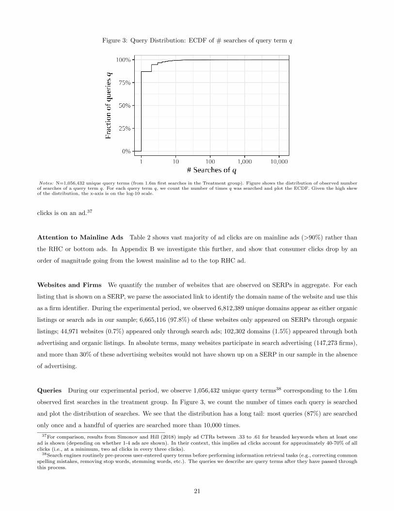
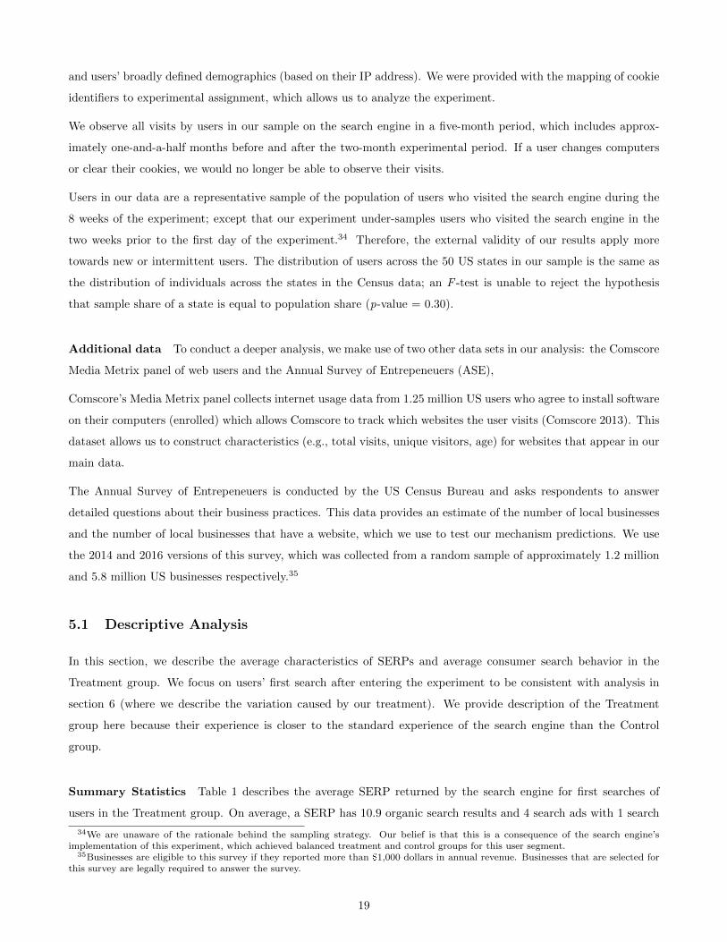
Figure 3: Query Distribution: ECDF of # searches of query term q

Notes: N=1,056,432 unique query terms (from 1.6m first searches in the Treatment group). Figure shows the distribution of observed numberof searches of a query term q. For each query term q, we count the number of times q was searched and plot the ECDF. Given the high skewof the distribution, the x-axis is on the log-10 scale.

clicks is on an ad.37

Attention to Mainline Ads Table 2 shows vast majority of ad clicks are on mainline ads (>90%) rather than

the RHC or bottom ads. In Appendix B we investigate this further, and show that consumer clicks drop by an

order of magnitude going from the lowest mainline ad to the top RHC ad.

Websites and Firms We quantify the number of websites that are observed on SERPs in aggregate. For each

listing that is shown on a SERP, we parse the associated link to identify the domain name of the website and use this

as a firm identifier. During the experimental period, we observed 6,812,389 unique domains appear as either organic

listings or search ads in our sample; 6,665,116 (97.8%) of these websites only appeared on SERPs through organic

listings; 44,971 websites (0.7%) appeared only through search ads; 102,302 domains (1.5%) appeared through both

advertising and organic listings. In absolute terms, many websites participate in search advertising (147,273 firms),

and more than 30% of these advertising websites would not have shown up on a SERP in our sample in the absence

of advertising.

Queries During our experimental period, we observe 1,056,432 unique query terms38 corresponding to the 1.6m

observed first searches in the treatment group. In Figure 3, we count the number of times each query is searched

and plot the distribution of searches. We see that the distribution has a long tail: most queries (87%) are searched

only once and a handful of queries are searched more than 10,000 times.

37For comparison, results from Simonov and Hill (2018) imply ad CTRs between .33 to .61 for branded keywords when at least onead is shown (depending on whether 1-4 ads are shown). In their context, this implies ad clicks account for approximately 40-70% of allclicks (i.e., at a minimum, two ad clicks in every three clicks).

38Search engines routinely pre-process user-entered query terms before performing information retrieval tasks (e.g., correcting commonspelling mistakes, removing stop words, stemming words, etc.). The queries we describe are query terms after they have passed throughthis process.

21

5.2 Randomization Checks

We conduct tests to check if the data are consistent with experimental randomization. First, we examine evidence

on whether users are assigned 50/50 to the experimental groups, and then we check whether users are similar on

pre-experiment observable characteristics.

On average, 49.98% proportion of our sample is assigned to the Treatment group, and this average is statistically

indistinguishable from 0.5 (two-sided t-test p-value = .37). We split our sample by the day when the user entered

our experiment, and conduct a similar test separately for each subsample. This gives us 56 p-values. We plot the

distribution function of these p-values in the left panel of Figure 4; using a Kolmogorov-Smirnov test we are unable

to reject that these p-values are coming from a uniform distribution between 0 and 1 (p-value = .58). We also

split our sample by the first query the user entered during the experimental period (for queries that were searched

more than 100 times in first searches) and conduct the same test. This provides us with 1,209 p-values and we plot

these values in the right panel of Figure 4; we are unable to reject that these p-values also come from a uniform

distribution (p-value = .21).

Figure 4: Randomization checks by day and query term

Notes: In the left panel, N=56 tests. In the right panel, N=1,209 tests. Figures show the distribution of p-values from testing that assignmentto the Treatment group happens with probability with 50%.The experiment’s randomization scheme predicts that 50% of users entering the experiment on each day of the experiment will be assigned to

the Treatment group. Similarly, 50% of users who search for any specific query term q should be assigned to the Treatment group. In the leftpanel, we plot the ECDF of the p-values from testing that assignment is random within a day. For each of the 56 days of the experiment, wetest that the percentage of users assigned to treatment is significantly different from .5. We cannot reject that these 56 p-values come from auniform distribution (p=.58). In the right panel, we do the same exercise by query. For each query q that was searched more than 100 timesin first searches (1209 unique queries), we test if 50% of users were assigned to Treatment. We cannot reject that these p-values come from auniform distribution (p=.21).

We are also able to observe some pre-experimental user behavior and we test that the experimental groups are

22

Table 3: Randomization checks for balance on observable characteristics

Variable AvgControl Std. DevControl AvgTreat Std. DevTreat p-value*

DateOfFirstExposure 27.35 16.14 27.36 16.13 0.59DRegisteredUser 0.135 0.34 0.135 0.34 0.47DManipulatedUser 0.105 0.31 0.105 0.31 0.88

DV isit 0.031 0.17 0.031 0.17 0.33log(1 + #V isits) 0.046 0.30 0.046 0.29 0.45log(1 + #AdClicks) 0.012 0.13 0.012 0.13 0.09log(1 + #OrganicClicks) 0.035 0.26 0.035 0.26 0.61log(1 + #DaysActive) 0.034 0.21 0.034 0.21 0.26log(1 + #V isits≥1MainlineAds) 0.030 0.22 0.030 0.22 0.31

DSearchForOtherSearchEngine 0.015 0.12 0.015 0.12 0.72

Notes: N=3,298,086 for all tests.*For each variable, p-values are from a two-sided t-test (with unequal variances assumption) for equality of means between Treatment

and Control groups.

Variable Descriptions: DateOfFirstExposure is the date a user entered the experiment and is calculated relative to the start of theexperimental period (i.e., it takes values from 0 to 55). DRegisteredUser indicates whether the user has created an account with thesearch engine. DManipulatedUser indicates whether or not, in their first search, the user entered a query on which our experiment actuallyvaried the number of ads (details on this are discussed in Appendix C). The remaining variables describe usage and click behavior in the1.5 months before the experiment (pre-experiment period). DV isit is an indicator for whether or not the user conducted any searches inthe pre-experiment period. #V isits, #AdClicks,#OrganicClicks denote the number of searches conducted on the search engine, clickson ad listings and clicks on organic listings in the pre-experiment period; #DaysActive indicates the number of days a user conducted atleast one search in the pre-experiment period; #V isits≥1MainlineAds indicates the number of SERPs shown to a user where the searchengine showed at least one mainline ad. We test these in terms of log one plus y. DSearchForOtherSearchEngine denotes whether a usermade at least one search that had the name of a competing search engine in its search terms before the beginning of the experiment.

balanced on these pre-experiment observables. Table 3 shows the results of these tests and we find that we cannot

reject that these groups are balanced.

6 Variation Caused by Experiment

How does advertising change the information presented to consumers? This is an important question because any

impact of advertising on consumer behavior is likely to occur through the ad’s impact on information presented

to consumers. To our knowledge, this question has not been answered empirically, because data on information

presented to or seen by consumers is typically unobserved. In this section, we first show that our experimental

treatment causes a change in the number of search ads seen by consumers. Then, we use data on the content of

ads and organic listings to show that the experimental treatment causes measurable changes in the information

presented to consumers. Since our objective in this section is to describe the change in information presented to

consumers conditional on searching, we focus on users’ first searches during our experiment. Searches subsequent to

the first one may be affected by the experimental treatment, and are therefore, not comparable between Treatment

and Control groups.39

6.1 Change in Mainline Ads

Table 4 reports the averages in the Control group (low prominence of advertising), and relative changes in search

ads and organic results presented on the SERP, going from control to treatment. In absolute terms, a Treatment

39Results on consumer behavior in section 7 are not limited to a single search.

23

group SERP presented .17 more mainline ads , .14 fewer RHC ads and .04 fewer organic results, on average, relative

to the Control group. This is expected as marginal ads that have ad scores above the mainline threshold τT and

below τC are moved to the RHC ad section, going from treatment to control. The changes in mainline ads and

RHC ads are not offsetting because, in some instances, the RHC ad section already has the maximum number of

ads in the Treatment group. In those situations, the marginal ad being moved from mainline to RHC crowds out

the lowest RHC ad.

There is a small but detectable change in the average number of organic listings seen as the result of the experiment.

This is likely due to heuristic rules regarding how many results may be shown in the entire mainline column. We

note that this effect is very small relative to both the effects on search ads and the size of the organic results section

(i.e., approximately 1 in 25 SERPs has 1 fewer organic search result in the Treatment group relative to the Control

group).

Table 4: Experimental Treatment — % Change in Ad and Organic Listings Shown

#MainlineAds #RHCAds #TotalAds #OrganicListings

Average in Control group* 0.83 1.69 3.98 10.95(Low ad prominence) (0.0012) (0.0015) (0.0033) (0.0038)

Average in Treatment group* 1.00 1.55 4.02 10.91(High ad prominence) (0.0012) (0.0014) (0.0034) (0.0038)

Percent Change** +20.52% -8.07% +1.05% -0.43%(from Control to Treatment) (0.18%) (0.08%) (0.08%) (0.03%)

p-value:H0 : No change between

Treatment and Control groups<.01 <.01 <.01 <.01

N 3,298,086 3,298,086 3,298,086 3,298,086

Notes: Table shows the average number of ad and organic listings shown to users in the Treatment and Control groups and thepercent change in listings shown going from Control to Treatment. Standard errors are shown in parentheses. A unit of observationis the first search conducted by a user during the experimental period. Each column shows the results for a different type of listing;#TotalAds is the sum of #MainlineAds, #RHCAds, #BottomAds.*

Averages are calculated over first searches conducted by users in the Control group (N=1,649,858 users) and in the Treatmentgroup (N=1,648,228 users).**

”Percent Change” is estimated by regressing the number of listings against an indicator for being in the Treatment group andtransforming the coefficient into a relative change. Standard errors are calculated using the delta method and robust to heteroskedas-ticity.

On average, there are 20.52% more mainline ads in the treatment group relative to the control group. Users in the

Treatment group see 1.05% more total search ads (i.e., combined mainline, RHC and bottom ads) and <1% fewer

organic search results on average.

Change in distribution of ads Since not all SERPs are affected by our experimental treatment (as discussed

in section 4.1), we also report the change in the distribution of mainline advertising on SERPs. Table 5 describes

the distribution of mainline ads across SERPs in Treatment and Control groups in the sample of first searches.

24

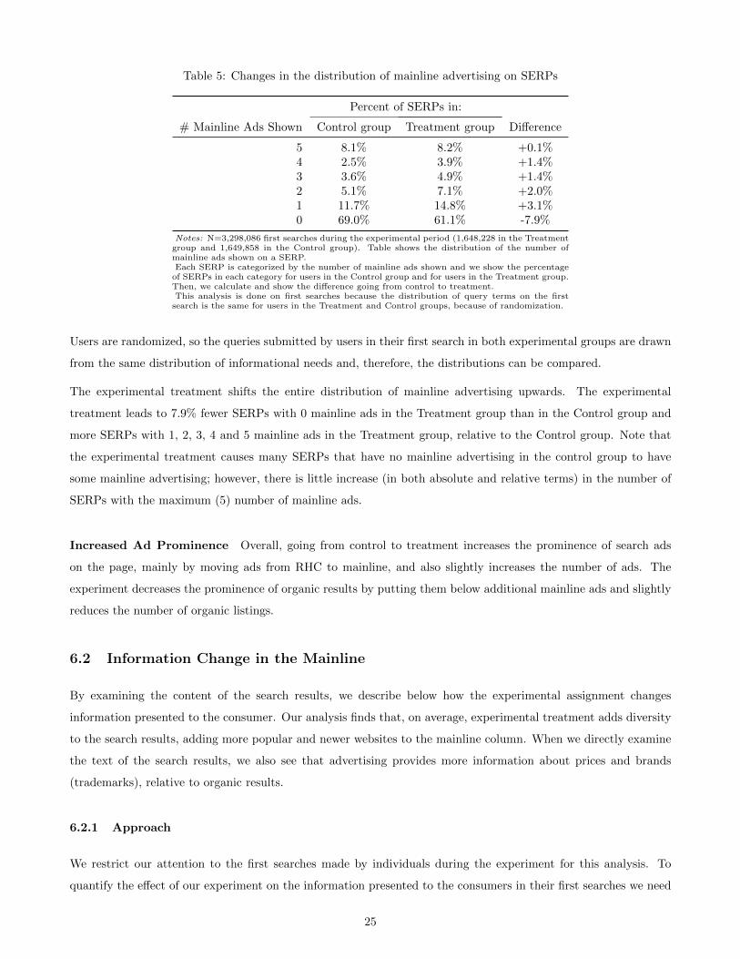
Table 5: Changes in the distribution of mainline advertising on SERPs

Percent of SERPs in:

# Mainline Ads Shown Control group Treatment group Difference

5 8.1% 8.2% +0.1%4 2.5% 3.9% +1.4%3 3.6% 4.9% +1.4%2 5.1% 7.1% +2.0%1 11.7% 14.8% +3.1%0 69.0% 61.1% -7.9%

Notes: N=3,298,086 first searches during the experimental period (1,648,228 in the Treatmentgroup and 1,649,858 in the Control group). Table shows the distribution of the number ofmainline ads shown on a SERP.Each SERP is categorized by the number of mainline ads shown and we show the percentage

of SERPs in each category for users in the Control group and for users in the Treatment group.Then, we calculate and show the difference going from control to treatment.This analysis is done on first searches because the distribution of query terms on the first

search is the same for users in the Treatment and Control groups, because of randomization.

Users are randomized, so the queries submitted by users in their first search in both experimental groups are drawn

from the same distribution of informational needs and, therefore, the distributions can be compared.

The experimental treatment shifts the entire distribution of mainline advertising upwards. The experimental

treatment leads to 7.9% fewer SERPs with 0 mainline ads in the Treatment group than in the Control group and

more SERPs with 1, 2, 3, 4 and 5 mainline ads in the Treatment group, relative to the Control group. Note that

the experimental treatment causes many SERPs that have no mainline advertising in the control group to have

some mainline advertising; however, there is little increase (in both absolute and relative terms) in the number of

SERPs with the maximum (5) number of mainline ads.

Increased Ad Prominence Overall, going from control to treatment increases the prominence of search ads

on the page, mainly by moving ads from RHC to mainline, and also slightly increases the number of ads. The

experiment decreases the prominence of organic results by putting them below additional mainline ads and slightly

reduces the number of organic listings.

6.2 Information Change in the Mainline

By examining the content of the search results, we describe below how the experimental assignment changes

information presented to the consumer. Our analysis finds that, on average, experimental treatment adds diversity

to the search results, adding more popular and newer websites to the mainline column. When we directly examine

the text of the search results, we also see that advertising provides more information about prices and brands

(trademarks), relative to organic results.

6.2.1 Approach

We restrict our attention to the first searches made by individuals during the experiment for this analysis. To

quantify the effect of our experiment on the information presented to the consumers in their first searches we need

25

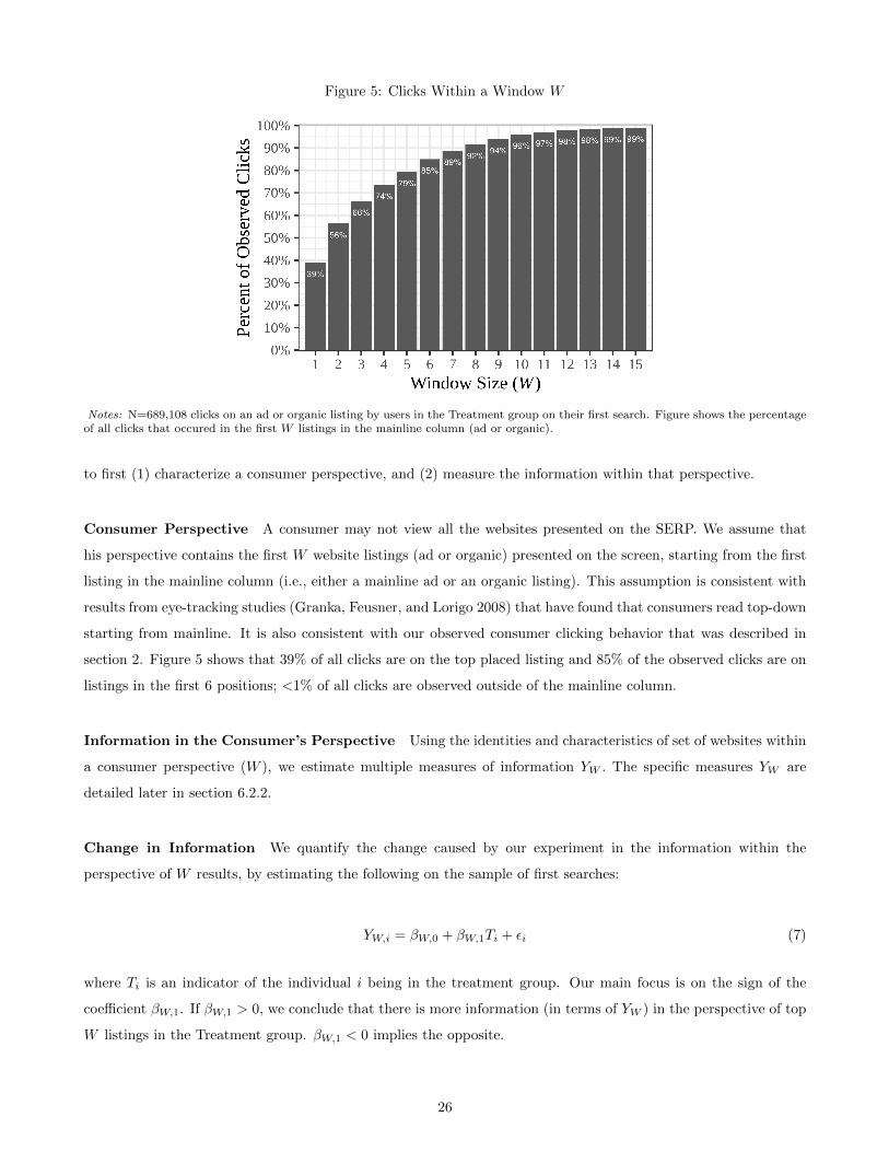
Figure 5: Clicks Within a Window W

Notes: N=689,108 clicks on an ad or organic listing by users in the Treatment group on their first search. Figure shows the percentageof all clicks that occured in the first W listings in the mainline column (ad or organic).

to first (1) characterize a consumer perspective, and (2) measure the information within that perspective.

Consumer Perspective A consumer may not view all the websites presented on the SERP. We assume that

his perspective contains the first W website listings (ad or organic) presented on the screen, starting from the first

listing in the mainline column (i.e., either a mainline ad or an organic listing). This assumption is consistent with

results from eye-tracking studies (Granka, Feusner, and Lorigo 2008) that have found that consumers read top-down

starting from mainline. It is also consistent with our observed consumer clicking behavior that was described in

section 2. Figure 5 shows that 39% of all clicks are on the top placed listing and 85% of the observed clicks are on

listings in the first 6 positions; <1% of all clicks are observed outside of the mainline column.

Information in the Consumer’s Perspective Using the identities and characteristics of set of websites within

a consumer perspective (W ), we estimate multiple measures of information YW . The specific measures YW are

detailed later in section 6.2.2.

Change in Information We quantify the change caused by our experiment in the information within the

perspective of W results, by estimating the following on the sample of first searches:

YW,i = βW,0 + βW,1Ti + εi (7)

where Ti is an indicator of the individual i being in the treatment group. Our main focus is on the sign of the

coefficient βW,1. If βW,1 > 0, we conclude that there is more information (in terms of YW ) in the perspective of top

W listings in the Treatment group. βW,1 < 0 implies the opposite.

26

The following example further clarifies our approach. Consider a situation in which the consumer searches for

“ebay shoes.” In the Treatment group the search engine presents eBay’s ad in the top mainline position, followed

by ebay.com as the first organic listing, and zappos.com as the second organic listing. In the Control group, eBay’s

ad is shifted to the right hand column, and the organic listing remains the same. If consumers view only the top

two results, a consumer in the treatment group is exposed to two listings from ebay (one ad, and one organic). A

consumer in the control group is exposed to one ebay and one zappos listing. Our approach compares information

in the sets {ebay.com; ebay.com}, and {ebay.com, zappos.com}. As there is no generally accepted value of W ,

we consider multiple values of W to show how information changes based on assumptions about the size of the

consumer’s perspective.

6.2.2 Measures of Information Within Search Results

We specify three measures of information (YW ) based on the identity of the firm whose link is placed in the SERP:

� #Unique Websites – One measure of information is the presence of a website within the consumer’s view.

To quantify this, we examine the URL associated with each listing, identify the website domain (e.g., ’ama-

zon.com’, ’espn.com’, etc.), and then calculate the number of unique domains within window W

YW = |{Domainp|∀p ≤W}|

where Domainp is the identity of the website in position p.

� Popularity – For each website we construct a measure of the popularity of a website (TotalV isits) by

calculating the number of visits by US users to the website in the year prior to our experiment using the

Comscore Media Metrix panel (see section 5). Then, for each SERP, and each level of window size W we

calculate:

YW = log

(1 +

1

W

W∑p=1

TotalV isitsp

)

where TotalV isitsp is the number of total visits observed in the Comscore data for the website in position p.

� Recency – We also construct a measure of how new a website is (Recency) by calculating the average time

when a user discovered the website in the Comscore panel.40 For every website, and each user who visited

the website at least once, we find the timestamp of the first visit. Then, we calculate the average of these

times. For interpretability, we calculate the deciles of this measure (RecencyDecile) over all the observed

websites, where the highest decile (10) corresponds to the website whose users started using it most recently.

We are able to create this measure for 1,427,410 websites, which covers 88.8% of all the clicks by users in

our sample of first searches. Sites that are not observed in the Comscore web panel are classified as being in

the highest decile for this analysis. Then, for each SERP, we calculate the average of RecencyDecile for the

40A direct measure of a website’s “age” is not available in any dataset we know of.

27

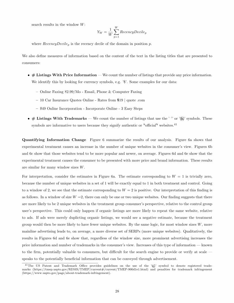
search results in the window W :

YW =1

W

W∑p=1

RecencyDecilep

where RecencyDecilep is the recency decile of the domain in position p.

We also define measures of information based on the content of the text in the listing titles that are presented to

consumers:

� # Listings With Price Information — We count the number of listings that provide any price information.

We identify this by looking for currency symbols, e.g. ’$’. Some examples for our data:

– Online Faxing $2.99/Mo - Email, Phone & Computer Faxing

– 10 Car Insurance Quotes Online - Rates from $19 | quote .com

– $49 Online Incorporation - Incorporate Online - 3 Easy Steps

� # Listings With Trademarks — We count the number of listings that use the ’�’ or ’®’ symbols. These

symbols are informative to users because they signify authentic or "official" websites.41

Quantifying Information Change Figure 6 summarize the results of our analysis. Figure 6a shows that

experimental treatment causes an increase in the number of unique websites in the consumer’s view. Figures 6b

and 6c show that those websites tend to be more popular and newer, on average. Figures 6d and 6e show that the

experimental treatment causes the consumer to be presented with more price and brand information. These results

are similar for many window sizes W .

For interpretation, consider the estimates in Figure 6a. The estimate corresponding to W = 1 is trivially zero,

because the number of unique websites in a set of 1 will be exactly equal to 1 in both treatment and control. Going

to a window of 2, we see that the estimate corresponding to W = 2 is positive. Our interpretation of this finding is

as follows. In a window of size W =2, there can only be one or two unique websites. Our finding suggests that there

are more likely to be 2 unique websites in the treatment group consumer’s perspective, relative to the control group

user’s perspective. This could only happen if organic listings are more likely to repeat the same website, relative

to ads. If ads were merely duplicting organic listings, we would see a negative estimate, because the treatment

group would then be more likely to have fewer unique websites. By the same logic, for most window sizes W , more

mainline advertising leads to, on average, a more diverse set of SERPs (more unique websites). Qualitatively, the

results in Figures 6d and 6e show that, regardless of the window size, more prominent advertising increases the

price information and number of trademarks in the consumer’s view. Increases of this type of information — known

to the firm, potentially valuable to consumers, but difficult for the search engine to provide or verify at scale —

speaks to the potentially beneficial information that can be conveyed through advertisement.

41The US Patent and Trademark Office provides guidelines on the use of the ’®’ symbol to denote registered trade-marks (https://tmep.uspto.gov/RDMS/TMEP/current#/current/TMEP-900d1e1.html) and penalties for trademark infringement(https://www.uspto.gov/page/about-trademark-infringement).

28

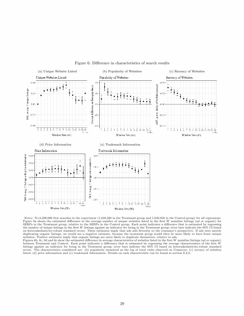
Figure 6: Difference in characteristics of search results

(a) Unique Website Listed (b) Popularity of Websites (c) Recency of Websites

(d) Price Information (e) Trademark Information

Notes: N=3,298,086 first searches in the experiment (1,648,228 in the Treatment group and 1,649,858 in the Control group) for all regressions.Figure 6a shows the estimated difference in the average number of unique websites listed in the first W mainline listings (ad or organic) forSERPs in the Treatment group, relative to the SERPs in the Control group. Each point indicates a difference that is estimated by regressingthe number of unique listings in the first W listings against an indicator for being in the Treatment group; error bars indicate the 95% CI basedon heteroskedasticity-robust standard errors. These estimates imply that ads add diversity to the consumer’s perspective. If ads were merelyduplicating organic listings, we would see a negative estimate, because the treatment group would then be more likely to have fewer uniquewebsites. Positive estimates imply that organic listings are more likely to duplicate themselves, relative to ads.Figures 6b, 6c, 6d and 6e show the estimated difference in average characteristics of websites listed in the first W mainline listings (ad or organic)between Treatment and Control. Each point indicates a difference that is estimated by regressing the average characteristics of the first Wlistings against an indicator for being in the Treatment group; error bars indicate the 95% CI based on heteroskedasticity-robust standarderrors. The characteristics considered are: (b) popularity measured as the log of total visits observed on Comscore, (c) recency of websiteslisted, (d) price information and (e) trademark information. Details on each characteristic can be found in section 6.2.2.

29

Table 6: Change in clicks due to experimental treatment

#AdClicks #OrganicClicks #TotalClicks

Average in Control group* 0.44 2.45 2.89(Low ad prominence) (0.029) (0.013) (0.032)

Average in Treatment group* 0.49 2.42 2.90(High ad prominence) (0.018) (0.012) (0.023)

Percent Change** 4.20% -0.78% 0.14%(from Control to Treatment) (0.16%) (0.13%) (0.13%)

p-value:H0: No change between

Treatment and Control groups

<.01 <.01 >.05

N 3,298,086 3,298,086 3,298,086

Notes: Table shows the average number of clicks on ad and organic listings in the Treatment and Controlgroups during the experimental period and the difference in clicks going from Control to Treatment. Eachcolumn shows the results for clicks on a different type of listing; #TotalClicks is the sum of #AdClicks and#OrganicClicks.*

There are N=1,649,858 users users in the Control group and N=1,648,228 users in the Treatment group.**

To calculate this, we regress log(1+y) against a indicator for being in the Treatment group. This allowsus to calculate percent change (reported) at the average level of y in the Control group; standard errors arecalculated using the delta method and robust to heteroskedasticity.

6.3 Discussion

In aggregate, we have shown that the experimental treatment has a measurable impact on both the prominence of

advertising that is shown during the experiment and the information presented to the consumer. Conditional on

searching, an average user in the Treatment group sees 20.52% more mainline ads, relative to Control. Furthermore,

if we assume that users have limited attention and only consider a subset of the results presented by the search

engine, additional advertising presents consumers, on average, more unique websites, newer websites and more

popular websites in their search results. In addition, additional advertising increases the price and trademark

information in the search results. In the next section we investigate whether this information change affects

consumer behavior in terms of clicks, and overall usage of the search engine.

7 Results – Consumer Behavior

7.1 Change in Clicks and Search Engine Revenue

Table 6 shows changes in user clicking behavior due to experimental assignment, aggregated over the entire ex-

perimental period of 8 weeks. It shows that users are more likely to click on ads when advertising prominence is

increased. Ad clicks increase and organic clicks decrease, indicating that consumers are substituting organic clicks

with ad clicks. In aggregate, we see a small and statistically insignificant increase in total clicks.

30

Table 7: Estimated impact on search engine revenue

Percentage ofLow Revenue Estimate* High Revenue Estimate* Ad Clicks Matched**

Control $747,958 $4,112,992 60.2%

Treatment $875,717 $4,297,378 60.0%

Difference +$127,759 +$184,385 +0.1%

% Difference +14.6% +4.3%

Notes: Table shows the estimated difference in search engine revenue during the experimental period (56 days)for the Treatment and Control group. Revenue estimates are based on Google Keyword Planner’s (GKP) Top ofPage Bids (low range and high range) from 11/2017 to 11/2018. For every ad click in the experiment, we find thecorresponding PPC using GKP and use this to estimate the revenue collected by the search engine. N=1,527,170ad clicks (725,739 in Control and 801,431 in Treatment).*"Low Revenue Estimate" is based on the 20th percentile of observed PPCs for a query q while "High Revenue

Estimate" is based on the 80th percentile. The procedure for calcuating these estimates is described in AppendixE.**

Unmatched clicks indicate that GKP had no historical bid estimates for the specified search query. For thepurpose of revenue estimation, we assume the PPC of unmatched clicks are $0.00.

Since search engine revenue depends on ad clicks, we expect search engine revenue to be higher in the Treatment

group, relative to Control. We do not have information on actual revenue paid to the search engine but we estimate

the change in revenue using publicly available data from Google Keyword Planner (GKP).42 We construct our

estimate in the following way. For every ad click that occurred in the Treatment and Control groups, we find the

query terms q that was associated with the ad click. Then, for each query term q, we use GKP to find the estimated

price per click (PPC). We match each ad click in our data with its estimated PPC to form our estimate of the

search engine’s revenue and aggregate for both the Treatment and Control.

We are able to match 60% of ad clicks in the Treatment group, and 60.2% of ad clicks in the Control group to

information from GKP.43 In Table 7, we estimate that search engine revenue increased between 4.3% and 14.6%

going from the Control to the Treatment group.

7.2 Search Engine Usage

The usage of the search engine in terms of total number of visits after entering the experiment is very heterogeneous

and skewed, with an average of 9.3 visits per individual in our sample, and the corresponding standard deviation

of 321.5 (min is 1 and max is 200,160). Table 8 shows various quantiles of the distribution.

Figure 7a shows the change in average number of visits to the search engine between the Treatment and Control

groups. For each individual, week 0 begins when an individual conducts their first search on the search engine

42Google Keyword Planner is a tool that allows practitioners to estimate the cost of running a search advertising campaign on Google.For any query q, GKP will provide the estimated price-per-click (PPC) for ads that were shown in the mainline section on Google.The tool provides a range of prices and are based on the realized prices for mainline ads over the last 12 months. Additional detailsare provided in Appendix E.

43Missing data indicates that the query terms q were either not observed frequently enough or did not have sufficient advertisingover the past 12 months for Google to form an estimate. For our estimate, we assume the revenue from these ad clicks are 0.

31

during the experimental time period (i.e., when the individual enters the experiment). In each of the 12 weeks

before and 12 weeks after an individual enters the experiment), we calculate the individual’s weekly usage (number

of searches conducted) of the search engine.44 We then compare the observed average usage of the search engine

in the treatment and control groups and plot the differences in Figure 7a.

As expected, there is little difference in average usage prior to the experiment. After entering the experiment, we

see that users in the Treatment group (who were likely to be presented more prominent advertising) increase their

search engine usage relative to Control in every week after entering the experiment. The increase is consistently

positive. In Figure 7b, we do the analogous exercise for the number of sessions initiated by users in the Treatment

and Control groups and find similar effects — Treatment group users consistently initiate more sessions, relative

to Control group users, after entering the experiment.

In aggregate, there are 2.47% more visits over the three months in the treatment group, relative to the control

group. Using a t-test we can reject the hypothesis that the average number of visits decreased with p-value=.04.

We can also reject that the average number of visits after the experimental time period decreased due to the

treatment (p-value=.015). For these tests we omitted top .05% outlier observations in terms of total number of

visits.45

To examine how the distribution of the number of visits changes due to the experimental treatment we estimate

quantile treatment effects (our approach follows Athey and Imbens 2017). This estimation is especially suitable for

our case because the distribution of number of visits is highly skewed, and estimating quantile treatment effects

limits the impact of outliers (Angrist and Pischke 2008, Chapter 7).

Table 9 presents changes in various quantiles between the Treatment and Control groups. Note that the 50th, 75th

and 90th quantiles do not change much across groups.46 We see a 2.1% - 2.3% increase in the higher quantiles.

The table also presents p-values from testing whether the quantiles of search engine usage decrease due to the

experimental treatment. These p-values are small, indicating little support for the hypothesis that search engine

usage decreased due to our treatment, at any level of the distribution. Figure 11 in the appendix plots changes in

other quantiles, and shows that none of the quantiles decreased due to the treatment.

As noted in section 6.1, not all individuals may be affected by the experimental variation because not all SERPs

have ads, and our experimental treatment may not change ad prominence on every eligible SERP. To examine the

change in usage of individuals we know who did experience the experimental variation, the table also presents the

same statistics for individuals whose first query during the experiment was one on which we know the experimental

treatment took place. For this subset of users, the effect is larger and still positive.47 This analysis shows that the

44Search engine usage is observed for up to 12 weeks after an individual enters the experiment. This does not mean, however, thatTreatment group individuals saw the experimental variation for 12 weeks. The experiment was active for 56 day and there are usersentering the experiment on each of the 56 days. This means that different cohorts of users were eligible for experimental treatment fordifferent amounts of time. The analysis in this section measures effects by considering all searches after the experiment begins (i.e., wepool a user’s usage during and after the experiment).

45Including these outliers increases the difference between treatment and control groups. The relative change from control totreatment in average number of visits is 0.55% without the outliers, and 2.47% when the outliers are included.

46Other researchers have also observed no change in lower quantiles due to treatment (e.g., see Athey and Imbens 2017).47Specifically, we identify queries for which the number of ads change significantly between treatment and control groups as ’manipu-

lated queries’. We then examine the subset of users who searched for a ’manipulated query’ in their first search during the experimentalperiod, as we know these users would have been affected by the experimental variationat least once. Details of this approach can befound in Appendix C.

32

Figure 7: Difference in search engine usage between treatment and control users by week

(a) Difference in Average # of Searches

(b) Difference in Average # of Sessions

Notes: N=3,298,086 users. Figures show the difference in search engine usage between users in the Treatment group and users in the Controlgroup, before and after they enter the experiment. The first time an individual visits the search engine during the experimental time period isset to week 0 (i.e., when the individual enters the experiment). Each bar is the difference in usage in terms of (a) average number of searchesand (b) average number of sessions, during one week.

33

Table 8: Difference in quantiles of usage between treatment and control group

(a) Total Visits, Full Sample

Quantile (s) Quantile in Control* Change*(τs) Rel. Change p-value** : H0 : τs < 0

50 3.00 0.00 0.0% <.00175 10.00 0.00 0.0% <.00190 10.00 0.00 0.0% <.00195 20.16 0.41 2.1% 0.069

99.5 127.61 2.88 2.3% 0.019

(b) Total Visits, subset of data with users who were exposed to experimental treatment in their first search.

Quantile (s) Quantile in Control* Change*(τs) Rel. Change p-value** : H0 : τs < 0

50 2.00 0.00 0.0% <.00175 4.00 0.00 0.0% <.00190 10.11 0.86 8.5% 0.00495 22.23 0.79 3.6% 0.004

99.5 169.85 15.48 9.1% 0.004

Notes: Tables show the quantile treatment effect (QTE) on TotalV isits at selected quantiles. We present results for (a) the fullsample (N=3,298,086 users) and (b) a subset of users who were exposed to the experimental treatment in their first search (N=345,310users). Details on identifying the subset can be found in Appendix C; more comprehensive QTEs can be found in Appendix D.*

We construct estimates from 10,000 bootstrap samples. We report the average level of the quantile in the control group from our10,000 bootstrap samples, i.e., ¯QY (0)(s), and, following the approach in Athey and Imbens (2017), we estimate the quantile treatmenteffect τs using the mean of the bootstrapped QTEs.**

This is the one-sided p-value, testing the null that the quantile treatment effect is negative, i.e. τs < 0.

treatment effect is present and larger where we expect it to be so.48

Table 9 shows a similar pattern in visits after the experimental variation ends. Higher quantiles of the distribution

of number of visits after the experiment increase due to the treatment, and none of the quantiles decrease.

Table 16 in Appendix D shows a similar pattern for the number of sessions. We find that the distribution of number

of sessions shifting to the right, going from Control to Treatment group, and see no evidence of decrease in the

number of sessions from making advertising more prominent.

Overall, we do not see evidence of usage decreasing in response to an increase in advertising prominence and

decrease in prominence of organic listings on the search engine. To the contrary, consumers appear to use the

search engine more when advertising is made more prominent.

7.3 Discussion

As laid out in section 2, our interpretation of these results is that, overall, consumers value the marginal ads

promoted by our experimental treatment; they value marginal ads as much as, or more than the marginal organic

listings. Our explanation is as follows. A user who faces an informational need must decide whether to use our

data partner’s search engine (’focal search engine’), or choose some outside option (no search, other informational

sources, competitor search engine). He decides based on his beliefs about the search engine’s quality (e.g., the

expected quality of the search results). Every time he conducts a search on the focal search engine, he updates his

48This analysis follows the literature on advertising field experiments (e.g., Johnson, Lewis, and Reiley 2016) which shows thatremoving “unaffected” individuals from the analysis increases statistical power.

34

Table 9: Difference in quantiles of post-experiment usage between treatment and control group

(a) Total Post Experiment Visits, Full Sample

Quantile (s) Quantile in Control* Change*(τs) Rel. Change p-value** : H0 : τs < 0

50 0.00 0.00 0.0% <.00175 0.00 0.00 0.0% <.00190 0.00 0.00 0.0% <.00195 1.00 0.00 0.0% <.001

99.5 54.86 1.58 2.9% 0.01

(b) Total Post Experiment Visits, subset of data with users who were exposed to experimental treatment in their first search.

Quantile (s) Quantile in Control* Change*(τs) Rel. Change p-value** : H0 : τs < 0

50 0.00 0.00 0.0% <.00175 0.00 0.00 0.0% <.00190 0.21 0.79 368.8% <.00195 4.02 0.77 19.2% 0.003

99.5 84.91 8.45 9.9% 0.007

Notes: Tables show the quantile treatment effect (QTE) on TotalV isits after the experimental variation ended at selected quantiles.We present results for (a) the full sample (N=3,298,086 users) and (b) a subset of users who were exposed to the experimental treatmentin their first search (N=345,310 users). Details on identifying the subset can be found in Appendix C; more comprehensive QTEs canbe found in Appendix D.*

We construct estimates from 10,000 bootstrap samples. We report the average level of the quantile in the control group from our10,000 bootstrap samples, i.e., ¯QY (0)(s), and, following the approach in Athey and Imbens (2017), we estimate the quantile treatmenteffect τs using the mean of the bootstrapped QTEs.**

This is the one-sided p-value, testing the null that the quantile treatment effect is negative, i.e. τs < 0.

beliefs based on the usefulness of the search result page he receives. In the treatment group, relative to the control

group, advertising is made more prominent, which increases the likelihood of seeing ads and reduces the likelihood

of seeing organic listings. Overall, consumers find marginal ads as much as, or more useful than marginal organic

listings. If marginal ads were less useful than the marginal organic listings, the consumers in the treatment group

would have had lower expectations from the search engine, and reduced their usage of it. However, we find no such

pattern.

As discussed in section 2, the increase in consumer usage of search engine in the Treatment group can also be

explained by the following alternative explanation. It is possible that consumers face high switching costs and do

not switch away to other search engines in the Treatment group even if they dislike prominent advertising. More

prominent advertising may cause increased search usage because users must now run more searches to find what

they are looking for.

This alternative explanation would predict that after the experimental time period, when the experimental variation

in advertising ceases to exist, the search engine usage pattern would be the same in the control and treatment groups

(as in the pre-experimental period). However, in Figures 7a and 7b we see the difference in usage persists beyond

the experimental time period of eight weeks.

In the subsequent analysis we provide further evidence that is inconsistent with this alternative explanation. By

this explanation, users who face low switching costs should be most likely to reduce their search usage when ad

prominence is increased. We test this prediction in the data in section 7.4. In section 7.5 we provide further

supporting analysis that shows that our effect is more likely to exist in situations where advertising is more useful

35

relative to organic results.

7.4 Focus on Marginal Individuals

We identify individuals who have searched for a different search engine before entering the experiment. These

individuals are aware of a competing search engine, and have switching costs low enough that they were willing to

navigate away to it in the past. Therefore, these individuals are less likely to tolerate any additional cost imposed

by advertising, relative to users who face higher switching costs.49 If our effects are driven by the alternative expla-

nation where individuals are stuck with worse search results, we would expect this subset of marginal individuals

to show a lower (more negative) response to our experimental treatment.

We examine this pattern in our data following the rationale in section 2.2.2, and conduct the following regression

log(TotalVisitsi) =β0 + β1Ti + β2Past Search For Competitori (8)

+ β3Past Search For Competitori × Ti + εi.

The dependent variable log(TotalVisiti) is the logarithm of the number of visits (searches) i made to the search en-

gine after experimental assignment; Ti is an indicator of i being in the treatment group; Past Search For Competitori

is an indicator of i searching for a competing search engine prior to the experiment; β’s are estimated regression

coefficients; εi is the idiosyncratic error term. Our focus is on β3 which estimates the difference in the treatment

effects for marginal individuals and the rest of the population, and β1 + β3 which is the effect of the treatment on

marginal individuals.

Results in column (1) of Table 10 indicate β3 > 0, that is, the marginal individuals are more likely to increase

their usage in response to advertising prominence, relative to the rest of the population. Further, we find that the

estimate of β1 + β3 is positive (two-sided, p-value = .024). Column (2) of the same table shows a similar pattern

when we focus only on post-experimental usage.

7.5 Additional Supporting Analysis to Describe the Main effect

In this section, we provide supporting analysis that shows that our effects are more likely when (a) ads are useful

and (b) organic listings are less useful.

7.5.1 Ad Usefulness and Usage

If the increase in visits caused by the experimental treatment occurs because the promoted ads make the content of

the search results page more useful to the consumer, we expect increase in usage to be positively correlated with an

increase in ad clicks. This prediction assumes that an ad click is a proxy for the ad being relevant to the individual.

49Our approach does not identify every marginal individual because individuals may reach another search engine through differentmeans. Therefore, our test compares marginal individuals with those not necessarily on the margin.

36

Table 10: Difference of Treatment effect on marginal users.

(1) DV: log visitsafter entering

experiment

(2) DV:log(1+visits afterexperiment ends)

Coef Se Coef Se

Treatment 0.0002 0.0013 .0007 .0006

Past Search For Competitor* -0.0122 0.0077 .2510 .0056

Treatment x Past Search For Competitor* 0.0246 0.0110 .0144 .0081

Intercept 1.1660 0.0009 .1111 .0004

N 3,298,086 3,298,086

Notes: Table shows regression results with standard errors that are robust to heteroskedasticity. Bolded coefficientsindicate p < 0.1. There are 50,950 users (1.5%) identified as having a prior knowledge of a search competitor.*"Past Search For Competitor" is an indicator for whether the user has been observed, before the experiment, con-

ducting a search for another search engine (i.e., a competitor of the focal search engine).

We cannot estimate an increase in ad clicks or an increase in usage at the individual level, so we cannot conduct

this analysis at the individual level (because one individual is observed in one experimental group only). Therefore,

we group individuals by the first query q they submitted to the search engine during the experiment. Let Sq be

the set of individuals whose first search during the experiment was for query q. For each query q, we estimate

1. the change in clicks on mainline ads caused by the experimental treatment for individuals in Sq:

∆ad clicksq =E(mainline ad clicks on first SERP|i ∈ Sq, i ∈ Treatment) (9)

− E(mainline ad clicks on first SERP|i ∈ Sq, i ∈ Control)

2. and, the change in search engine visits caused by the treatment for individuals in Sq:

∆visitsq =E(visits to the search engine|i ∈ Sq, i ∈ Treatment) (10)

− E(visits to the search engine|i ∈ Sq, i ∈ Control)

A higher ∆ad clicksq signifies more relevant ads are made prominent by the experiment. Therefore, we expect the

treatment effect on usage of the search engine to be higher when ∆ad clicksq is higher. That is, ∆ad clicksq and

∆visitsq are expected to be positively correlated.

We estimate ∆ad clicksq and ∆visitsq for 13,076 queries, and find a positive correlation (r=.036; p<.01) between

the measures.

Further Analysis We categorize queries based on whether we observe a statistically significant increase in

clicks caused by our experiment in individuals in Sq. Column (1) of Table 11 shows that in instances where the

experimental treatment causes an increase in clicks (i.e., ∆ad clicksq > 0), it also increases consumers’ usage of

37

Table 11: Correlation between change in ad clicks and change in search engine usage

(1) q: ad clicks increaseddue to treatment

(2) q: no ad clicksincrease due to treatment

Change inlog(TotalV isits)

.0460 (.0197) .0034 (.0033)

Change inlog(1 + V isitsOnSameDay)

.0078 (.0125) .0031 (.0026)

Change inlog(1 + V isitsAfterADay)

.0408 (.0152) -.0008 (.0023)

Notes: Table shows averages and standard errors in parentheses. N=13,076 queries (359 with ad click increase detected,and 12,717 with no ad click increase detected).We group individuals based on the first query (q) they typed during the experiment into subsets Sq . For each Sq we estimate

the change in mainline ad clicks (∆ad clicksq) between treatment and control groups. Column (1) uses data for i ∈ Sq suchthat ∆ad clicksq>0; two-sided test of significance of ∆ad clicksq has a t-stat>1.6 ; column (2) uses data for i ∈ Sq suchthat ∆ad clicksq 6> 0; point estimate of ∆ad clicksq < 0, or two-sided test of significance of ∆ad clicksq has a t-stat<1.6.For different subsets of data, row 1 reports the change between treatment and control in log of total visits after entering theexperiment; row 2 reports the change between treatment and control in log of visits during the same day when the user typedq; row 3 reports the change in log of future visits. Across columns, we observe that an indicator of a statistically significantincrease in ∆ad clicksq is correlated with change in log of total visits (p=.033), and change in log of visits after a day (p<.01),but not with change in log of visits within a day (p=.71).

the search engine (∆visitsq > 0). Most of the increase in usage occurs in the future as we see no evidence of

increase in usage on the same day (which is the user’s first day in the experiment). In Column (2), we see that in

instances where the experimental treatment causes no increase in clicks, treatment effect on search engine usage is

also insignificant. Across columns, we observe that an indicator of a statistically significant increase in ∆ad clicksq

is correlated with change in log of total visits (p=.033), and change in log of visits after a day (p<.01), but not

with change in log of visits within a day (p=.71).

7.5.2 Organic Listings and Usage

The experimental treatment increases the prominence of advertising and decreases the prominence of organic

results. Therefore, we expect the experimental treatment to be more useful to individuals in situations where the

organic listings are less useful. In this section, we aim to test this prediction by examining how the treatment effect

varies with the nature of information in organic listings presented to individuals. We first construct two measures

that proxy for relevance of the organic listings and then we analyze how the treatment effect varies across these

measures.

Measuring Usefulness of Marginal Organic Listing For every query q, we construct two measures that

proxy for the usefulness of the marginal organic listing that potentially gets displaced when the marginal search

ad gets placed in the mainline because of the experiment. First, we construct a measure of the variety in a

query’s organic listings based on the concentration of pre-experimental organic clicks across the listed websites. For

each query, we estimate the share of historical clicks going to each listed website, and calculate a three-firm HHI

(Herfindahl Index).50 A query has an HHI of 1 when all organic clicks have been going to one website, which means

50For each query, this is the sum of squares of click-share of top three websites.

38

that historically the search engine’s organic algorithm has directed all searches for this query to a single website.

Brand queries, which have been studied as a specific case in previous research, will have HHIs close to 1 as users

who search for brand queries will usually only click on the listing for the brand’s website. A lower HHI generally

implies that the organic listings provide multiple options that are comparable in terms of their relevance to the

user’s query, because consumers click on a variety of websites.51 Plot (a) in figure 8 shows a histogram of HHI

across queries for which we have at least 10 historical clicks (to reliably estimate the HHI). The plot shows that

queries’ concentrations cover the entire range from 0 to 1. To simplify later interpretation, we split this measure

into quartiles. Brand queries, with HHIs close to 1, are represented by the highest quartile.

All else equal, we expect the value of adding an additional unique listing – as our experimental treatment does – is

higher when the organic results have organic listings that are concentrated on one website, as opposed to situations

when they are already diverse. Consequently, we would expect our treatment effect should be higher in situations

where organic results are more concentrated.

Secondly, we construct a measure of organic listing relevance based on historical clicking rates on organic listings.

If the search engine returns a search result page with low relevance organic listings, we assume that the consumers

would not have clicked on these listings and the organic clicks per search (i.e., the organic click rate, or OCR) on

this type of search result page will be low. For every query, we calculate the OCR and then we plot its histogram

in plot (b) of Figure 8. As this distribution appears multi-modal, we split this measure into deciles instead of

quartiles for the purpose of interpretation. We expect that reducing the prominence of organic results through

our experiment would be more agreeable to consumers when the query’s SERP has low OCR. This means that we

would expect larger benefit from advertising for users in lower deciles of OCR.

Analysis Setup In the following analysis, we examine how the experimental treatment effect varies with the

characteristics of the organic results the search engine historically returned for the query. As the number and the

nature of queries entered by an individual over the course of the experiment is endogenous, and may depend on

how they respond to the experimental treatment, we limit our focus to the first query the individual entered during

the experimental time period. This query is not affected by the experimental variation. This means that each

individual is matched to one query for this analysis.

To assess how the treatment effect varies with these measures, we run the following regression:

log(TotalVisitsi) = β0+β1Ti+

4∑q=2

β2,qHHIq,i+

10∑d=2

β3,dOCRd,i+

4∑q=2

γ1,qHHIq,i×Ti+

10∑d=2

γ2,dOCRd,i×Ti+εi. (11)

The dependent variable log(TotalV isitsi) is the logarithm of the total number of visits (searches) i made to the

search engine after entering the experiment; Ti is an indicator of i being in the treatment group; HHIq,i is an

indicator that the first query entered by i is in the q-th quartile of historical click HHI; OCRd,i is an indicator that

the first query entered by i is in the d-th decile of historical organic click rate (OCR). β’s and γ’s are estimated

51This measure captures the relevance-weighted variety of the organic listings. When there are a large number of listed websites,but only one is of high relevance (and is clicked), this measure would report high concentration whereas a measure based on just thenumber of listed websites would report low concentration.

39

Figure 8: Distribution of historical click concentration and organic click rate

(a) Distribution of Click Concentration (b) Distribution of Organic Click Rate

Notes: Figures show histograms of historical clicking behavior and associated quantile cutpoints (quartile and decile) used in the nextanalysis. For each user, we focus on the first query they typed during the experiment and calculate the historical concentration (HHI) ofclicks for the query and the historical click rate on any organic listing (OCR). We run this analysis for any query that received organicclicks from more than 10 users in our pre-experimental data. This allows us to calculate historical concentration and OCR for a subsampleof N=706,534 users (who submitted 49,931 unique queries).Figure (a) shows the distribution of the three-firm HHI; we show the separation of this distribution into 4 quartiles. Figure (b) presents thedistribution of the historical organic click rate, with OCR > 1.5 mapped to 1.5; we show the separation of this distribution into 10 deciles.

regression coefficients; εi is the idiosyncratic error term. Our focus is on the coefficient of the set of interaction

terms γ1,q and γ2,d, which estimate the effect in different quartiles/deciles of our measures.

Table 12 shows that the effect of the treatment is higher when the the user’s first query had a low organic click

rate, and when clicks tend to be concentrated. In Column (1) and Column (2), we show the partial specifications.

In Column (3), we show the full specification and find that that the treatment effect is highest when the organic

listings are highly concentrated (highest two quartiles). and when the query has historically low organic click rate

(the omitted decile). By conducting a joint test, we reject that the effect in the omitted decile is lower than in

any of the other deciles (p=.026). Our results also show that users who search for brand queries, captured by the

fourth quartile of HHI, increase their usage in response to the experimental increase in prominence of advertising.

8 Mechanism

Overall, our results are consistent with consumers getting higher utility from the placement of the marginal ad in a

prominent position, which reduces the prominence of organic listings. What does this tell us about the underlying

mechanism and the nature of the equilibrium in our context? What kinds of businesses benefit from advertising?

If the organic listings were a perfectly sorted list of most relevant websites, then making advertising more prominent

can only make the consumer worse off. The rationale for this statement is as follows: increasing the prominence

40

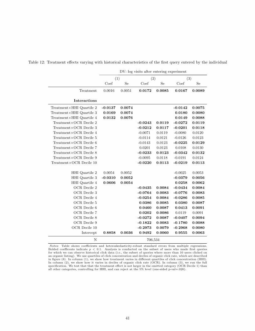
Table 12: Treatment effects varying with historical characteristics of the first query entered by the individual

DV: log visits after entering experiment

(1) (2) (3)

Coef Se Coef Se Coef Se

Treatment 0.0016 0.0051 0.0172 0.0085 0.0167 0.0089

Interactions

Treatment×HHI Quartile 2 -0.0137 0.0074 -0.0142 0.0075Treatment×HHI Quartile 3 0.0169 0.0074 0.0180 0.0080Treatment×HHI Quartile 4 0.0132 0.0076 0.0149 0.0088

Treatment×OCR Decile 2 -0.0243 0.0119 -0.0272 0.0119Treatment×OCR Decile 3 -0.0212 0.0117 -0.0201 0.0118Treatment×OCR Decile 4 -0.0071 0.0119 -0.0080 0.0120

Treatment×OCR Decile 5 -0.0114 0.0121 -0.0126 0.0123

Treatment×OCR Decile 6 -0.0143 0.0123 -0.0225 0.0129Treatment×OCR Decile 7 0.0201 0.0123 0.0108 0.0130

Treatment×OCR Decile 8 -0.0233 0.0123 -0.0342 0.0132Treatment×OCR Decile 9 -0.0095 0.0118 -0.0191 0.0124

Treatment×OCR Decile 10 -0.0220 0.0113 -0.0219 0.0113

HHI Quartile 2 0.0054 0.0052 -0.0025 0.0053

HHI Quartile 3 -0.0310 0.0052 -0.0379 0.0056HHI Quartile 4 0.0606 0.0054 0.0258 0.0062

OCR Decile 2 -0.0435 0.0084 -0.0434 0.0084OCR Decile 3 -0.0764 0.0083 -0.0776 0.0083OCR Decile 4 -0.0254 0.0084 -0.0286 0.0085OCR Decile 5 0.0386 0.0085 0.0380 0.0087OCR Decile 6 0.0460 0.0087 0.0413 0.0091OCR Decile 7 0.0202 0.0086 0.0119 0.0091

OCR Decile 8 -0.0272 0.0087 -0.0407 0.0094OCR Decile 9 -0.1822 0.0083 -0.1780 0.0088

OCR Decile 10 -0.2973 0.0079 -0.2968 0.0080Intercept 0.8858 0.0036 0.9492 0.0060 0.9555 0.0063

N 706,534

Notes: Table shows coefficients and heteroskedasticity-robust standard errors from multiple regressions.Bolded coefficents indicate p < 0.1. Analysis is conducted on the subset of users who made first queriesfor which we can observe historical click data (i.e., the subset of queries where more than 10 users clicked onan organic listing). We use quartiles of click concentration and deciles of organic click rate, which are describedin figure (8). In column (1), we show how treatment varies in different quartiles of click concentration (HHI).In column (2), we show how it varies in deciles of organic click rate (OCR). In column (3), we run the fullspecification. We test that that the treatment effect is not larger in the omitted category (OCR Decile 1) thanall other categories, controlling for HHI, and can reject at the 5% level (one-sided p-val=.026).

41

of advertising places an inferior link in a more visible position, therefore, consumers will have to spend more effort

to reach the relevant websites and satisfy their informational need. This would imply that consumers are worse off

when ads are made prominent.

Hence, the possibility of marginal ads providing higher utility than marginal organic listings implies that organic

listings are not perfect; the algorithm used to sort them has incomplete information, which can be complemented

with advertising.

In this section, we analyze the data to examine the existence of specific features of an equilibrium in which ads

help inform consumers by conveying advertisers’ private information.52 In our conceptualization, some firms have

information that (1) is private to them – unknown to the consumer or the search engine, and (2) conveying this

information makes the consumer more likely to pick the advertiser over other competing options. This private

information could be the existence of the firm, or its attributes. For example, consider a new grocery store A in a

location that home-delivers groceries locally at a low price. Consumers may not be aware of it. The search engine

may not have catalogued and evaluated store A’s website because it is new. In this case, the existence of store

A is privately known to the business, and the consumer may value knowing about it. In another situation, it is

possible that the consumer does not know about the store, but the search engine does know that it’s website exists.

However, the search engine is unsure whether store A is more relevant than other options (established grocery

chains) that appear in the organic listings. In this case the private information store A has is its high relevance

(because it delivers locally at a low price) to the consumer’s search need, which is known only to store A.

For simplicity, we denote the set of firms with such private information as N (for new, or lesser known firms),

and the others as K (for known). Appendix A lays out a model that makes behavioral predictions in this setting.

The intuition is as follows. Firms in N want to advertise because otherwise they would not be considered by

the consumer on the search engine. Among the N firms, the best firms are the ones that actually advertise in

equilibrium because they gain the most from advertising. They gain the most because they can reveal private

information (e.g., hidden characteristics) to consumers which makes consumers more likely to click on them.53 We

extend the above example to explain the intuition. Say, there are two new grocery stores A, and B home delivering

in an area. Both are unknown to the search engine. Stores A and B are very similiar except store B offers local

delivery at a higher price than store A. Store A is more likely to satisfy the consumer’s need than store B because it

provides home-delivery at a lower price. Stores A and B can both convey their existence to the consumer through

advertising, but A can also convey that it has lower price. Therefore, A benefits more from advertising than B,

and will advertise in equilibrium.

Overall, advertising makes consumers better off by adding useful new information to the search results page. It

makes consumers more likely to visit websites of N firms, because advertising makes consumers more aware of

them. Hence advertising benefits firms in N . Because the consumer is more likely to be satisfied when the search

52We do not say that conveying private information is the only motivation for advertising. Rather, we say that this mechanism drivesour finding of consumers preferring advertising.

53In situations where the firm’s private information is verifiable by the consumer before purchase, the ad simply conveys the verifiableinformation. For example, in a situation where the consumer and the search engine are unaware of the firm, the ad makes the consumeraware of it. In situations where the firm’s private information cannot be verified by the consumer before purchase, for example, whenthe firm sells a high quality experience good, advertising serves as a costly signal (as in Sahni and Nair 2018).

42

engine allows advertising, he is more likely to use the search engine in the future. In the rest of this section we

check for predictions implied by this mechanism in the data.54

Predictions We assume that newer websites are more likely to have private information that is unknown to the

search engine. This assumption is backed by our discussion of search engine data gathering algorithms, presented

in section 3.1. Empirically, we check the following in support of our proposed mechanism:

� Newer websites are more likely to engage in search advertising.

� Increasing the prominence of advertising increases traffic to newer websites.

� Advertising benefits the consumers more in markets with more new local websites. The comparative static

in Appendix A.5 analytically shows this prediction.

8.1 Analysis – advertising behavior

To assess the effect of the experiment on newer websites and advertisers, we create the following measures for each

website:

� RecencyDecile- This is a decile measure of the average time when a user discovered the website and is the

same as the measure of age we used in section 6.2. Higher values (e.g., 10) indicate newer websites.

� WebsiteAdvertised – An indicator of whether the website spent money on advertising, which is determined

by whether an ad click occurred on a website’s search ad

� ChangeInTraffic – The difference in the number of total clicks a website receives (organic + ad) from users

in the Treatment group, relative to the Control group. This is a measure of how the experimental variation

changes total traffic to a website.

This allows us to assess our first prediction about the relationship between advertising and website age by regressing

WebsiteAdvertised on our measure of the website’s age, RecencyDecile. Table 13 presents the regression. Column

(1) shows that newer websites are more likely to advertise. The coefficient of interest does not change significantly

when we add other characteristics of website usage (the number of unique visitors and the number of repeat users

to the website in the Comscore data) to the regression, as seen in column (2).

Do these newer websites also gain more from our experimental variation of advertising? To assess this, we regress

ChangeInTraffic on the website characteristics. Columns (3) and (4) of Table 13 show that newer websites are

the ones that benefit most from increasing advertising prominence on the search engine, relative to websites that

are older. This is consistent with our second prediction that advertising increases traffic to newer websites. In

relative terms, the newest decile of websites gains 9.7% more traffic from treatment group relative to control.

54One could conceptualize a different model, in which there is no unknown firm, or unknown firms are inferior in the sense that theywould not satisfy the consumer need. In such a model, the consumer would be weakly worse off in the presence of advertising, whichis contrary to our finding. We discuss this model further in section A.6.

43

Table 13: Advertising behavior of new websites

DV: WebsiteAdvertised DV: ChangeInTraffic

(1) (2) (3) (4)

RecencyDecile 0.0127 0.0129 0.1260 0.1286(0.0003) (0.0003) (0.0433) (0.0426)

Historic: # Unique visitors 0.0199 0.1197(0.0003) (0.0431)

Historic: % Repeat Users -0.0066 -0.0129

(0.0003) (0.0397)

Intercept 0.0488 -0.0220 -0.4492 -1.0473(0.0019) (0.0031) (0.2718) (0.3963)

N 137,523

Notes: Table shows coefficients and heteroskedasticity-robust standard errors from multipleregressions. Bolded coefficents indicate p < 0.1. A unit of observation is a website that was (a)presented on at least one SERP during the experimental period (56 days) and (b) a website forwhich we can generate historical characteristics using Comscore data (i.e., visited at least once onComscore).

8.2 Analysis – variation in presence of local and new websites

We examine the prediction that the consumer benefit from advertising increases when there are more websites with

private information. The presence of websites does not vary experimentally so, to assess how the presence of newer

websites changes the treatment effect, we use geographic variation (across states) in the presence of local businesses

with websites. We use data from the Annual Survey of Entrepeneurs, which was described in section 3.1.3, to

measure the percent of local businesses that have a website in each state. This percentage varies across states and

across time (from 2014 to 2016).

In Figure 9 we categorize states into quartiles based on the percent of local businesses that have their own websites.

We estimate the treatment effect on usage of the search engine seperately for individuals from these groups of states

and plot the effects in Figure 9. The figure shows that the treatment effect is largest among users in states with

the highest percentage of businesses having websites, and the effect increases significantly with quartile. In Table

14, we report the quantile treatment effects for each quartile and find the effects are largest in the fourth quartile,

relative to other quartiles.

Further Analysis To control for other factors and examine this further, we regress log of total visits to the

search engine after entering the experiment on the share of businesses in the user’s state that had a website in 2016.

The regression is presented in column (1) of Table 15 and supports that the effect of experimental assignment is

higher in states with a higher share of local business websites.

To investigate whether presence of newer websites causes this effect, we replace the share of businesses with a

website in 2016 with the share of of businesses with a website in 2014 and the change in the share between 2014

and 2016. Since ASE started in 2014, we cannot go further back in time. The share of businesses with website in

44

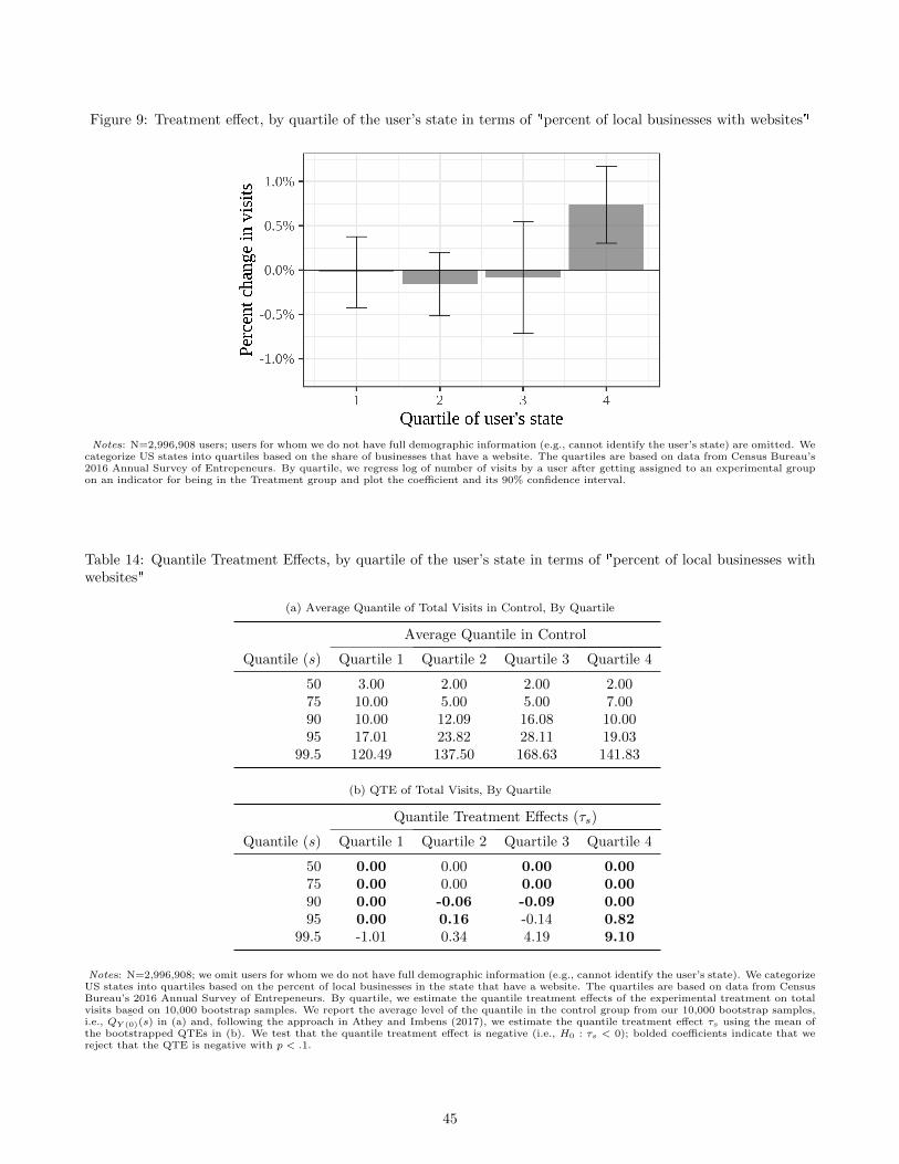
Figure 9: Treatment effect, by quartile of the user’s state in terms of "percent of local businesses with websites"

Notes: N=2,996,908 users; users for whom we do not have full demographic information (e.g., cannot identify the user’s state) are omitted. Wecategorize US states into quartiles based on the share of businesses that have a website. The quartiles are based on data from Census Bureau’s2016 Annual Survey of Entrepeneurs. By quartile, we regress log of number of visits by a user after getting assigned to an experimental groupon an indicator for being in the Treatment group and plot the coefficient and its 90% confidence interval.

Table 14: Quantile Treatment Effects, by quartile of the user’s state in terms of "percent of local businesses withwebsites"

(a) Average Quantile of Total Visits in Control, By Quartile

Average Quantile in Control

Quantile (s) Quartile 1 Quartile 2 Quartile 3 Quartile 4

50 3.00 2.00 2.00 2.0075 10.00 5.00 5.00 7.0090 10.00 12.09 16.08 10.0095 17.01 23.82 28.11 19.03

99.5 120.49 137.50 168.63 141.83

(b) QTE of Total Visits, By Quartile

Quantile Treatment Effects (τs)

Quantile (s) Quartile 1 Quartile 2 Quartile 3 Quartile 4

50 0.00 0.00 0.00 0.0075 0.00 0.00 0.00 0.0090 0.00 -0.06 -0.09 0.0095 0.00 0.16 -0.14 0.82

99.5 -1.01 0.34 4.19 9.10

Notes: N=2,996,908; we omit users for whom we do not have full demographic information (e.g., cannot identify the user’s state). We categorizeUS states into quartiles based on the percent of local businesses in the state that have a website. The quartiles are based on data from CensusBureau’s 2016 Annual Survey of Entrepeneurs. By quartile, we estimate the quantile treatment effects of the experimental treatment on totalvisits based on 10,000 bootstrap samples. We report the average level of the quantile in the control group from our 10,000 bootstrap samples,i.e., ¯QY (0)(s) in (a) and, following the approach in Athey and Imbens (2017), we estimate the quantile treatment effect τs using the mean ofthe bootstrapped QTEs in (b). We test that the quantile treatment effect is negative (i.e., H0 : τs < 0); bolded coefficients indicate that wereject that the QTE is negative with p < .1.

45

2014 represents the presence of “local websites” – businesses in the user’s state that have a website older than two

years at the time of the experiment. The change in share between 2014 and 2016 gives us a measure of “new” local

websites. When we add these measures to the regression, along with their interaction with the treatment indicator,

we see that the increase in usage due to advertising prominence is driven by the presence of new local websites.

The growth of local business websites may be correlated with other factors that change over time. It is possible

that states with high growth of local business websites are also growing overall, which increases the utility from

advertising in other ways. To control for this, we add income related measures – state-level GDP growth between

2014 and 2016, and the level of per capita income in the state – to the regression to control for such factors. Column

(3) shows that the coefficients corresponding to the interaction between treatment indicator and change in share

of local businesses with websites between 2014 and 2016 remains similar. Advertising may also be less useful for

younger users, who are more likely to read reviews. In Column (4), we control for the median age of the state and

find that there is not substantial difference in the treatment effect based on the median age of the stage.

Overall, we conclude from this analysis that increased presence of newer local businesses with websites increases

the benefit from advertising. This finding is consistent with an equilibrium in which advertising allows lesser known

businesses reach consumers.

9 Conclusion

This study analyzes a large-scale experiment conducted on a US search engine that experimentally varied the

prominence of search advertising. The experiment allows us to directly test whether advertising supplied on the

search engine provides positive value to consumers, or not. Our experimental treatment increases the prominence

of advertising, which increases consumer clicks on ads and reduces clicks on organic listings. Analyzing revealed

preference data, we find that consumers value the marginal ads as much as, or higher than marginal organic listings

on average. Overall, we see no evidence of consumers aversion to the experimental treatment; marginal consumers

prefer it. From the perspective of the search engine, our effects are also economically significant — showing more

prominent ads leads to the search engine collecting 4.3-14.6% more revenue. In our analysis we do not see an

incentive for the search engine to reduce search advertising from the current status quo level. By compensating

with information that is missed out by organic listing, search advertising seems to attract users rather than driving

them away from the search engine. Unlike much of the literature on advertising, our focus is not on how exposure

to an ad changes consumer behavior with respect to the advertiser. Rather, we study consumers’ overall valuation

of search advertising.

Our data support the view that search advertising encourages competition. Search engines assess the relevance

of websites based on indirect signals that are difficult for new websites to obtain. Therefore, newer websites are

less likely to be presented to consumers, relative to older websites, in the organic listings even when they are more

relevant to consumer search needs. Search advertising provides a means for new and relevant websites to reach

consumers, thereby improving the overall information presented to consumers.

46

Table 15: Variation in the treatment effect with presence of new local business websites

DV: log of total visits after entering experiment

(1) (2) (3) (4)

Treatment -0.0280 -0.0324 -0.2010 -0.2031

(0.0128) (0.0141) (0.1306) (0.1259)

Treatment × 2016 Share of firms with websites 0.0535(0.0231)

Treatment × 2014 Share of firms with websites 0.0561 0.0468 0.0468(0.0247) (0.0252) (0.0263)

Treatment × Change in share from 2014 to 2016 0.2252 0.2660 0.2920(0.1296) (0.1266) (0.1409)

Treatment × GDP growth from 2014 to 2016 0.0173 0.0185

(0.0368) (0.0374)

Treatment × Log per capita income 0.0178 0.0192

(0.0133) (0.0130)

Treatment × Median Age -0.0005

(0.0005)

2016 Share of firms with websites -3.5222

(3.1335)

2014 Share of firms with websites -3.3610 -2.7666 -2.3546

(2.9632) (2.3238) (2.0604)

Change in share from 2014 to 2016 5.4764 3.2708 7.8723

(8.3090) (11.3232) (10.6229)

GDP growth from 2014 to 2016 1.4423 2.1517

(2.7113) (2.3809)

Log per capita income -0.3283 -0.0586

(0.6900) (0.6083)

Median Age (State) -0.0610(0.0269)

Intercept 2.9816 2.7443 5.8910 5.1858

(1.7729) (1.6807) (7.6554) (6.9313)

N* 2,996,908

Notes: Table shows coefficients and standard errors from multiple regressions; standard errors are clustered by state.Bolded coefficents indicate p < 0.1. A unit of observation is a single user.*

We omit users for whom we do not have full demographic information (e.g., cannot identify the user’s state).

47

More generally, our findings indicate users are not passive consumers of information supplied to them. They provide

feedback to the media on the quality of information it shows them, which is an essential economic force for markets

to supply good information in the long term (DellaVigna and Gentzkow 2010).

Future work can investigate whether our findings extend to other ad-supported media contexts, such as TV and

radio. In those contexts, advertising is often understood as a pseudo-price paid by consumers for free media

(Anderson and Coate 2005). If the search engine marketplace is unique in supplying useful advertising to consumers,

why would that be? Is it because ads are better targeted, or because there are low fixed costs for small advertisers,

or some other reason? These are interesting questions for future research.

References

Abernethy, Avery M and George R Franke (1996). “The information content of advertising: A meta-analysis”. In:

Journal of advertising 25.2, pp. 1–17.

Ackerberg, Daniel A. (2001). “Empirically distinguishing informative and prestige effects of advertising”. In: RAND

Journal of Economics, pp. 316–333.

ACSI (July 2018). U.S. customer satisfaction with internet portals and search engines in 2018 (index score). url:

https://www.statista.com/statistics/273900/user- satisfaction- with- us- internet- portals/

(visited on 03/09/2019).

Aiello, Luca et al. (2016). “The Role of Relevance in Sponsored Search”. In: Proceedings of the 25th ACM Interna-

tional on Conference on Information and Knowledge Management. ACM, pp. 185–194.

Alphabet, Inc. (Feb. 2019). 2018 Form 10-K Annual Report. https://abc.xyz/investor/static/pdf/20180204_

alphabet_10K.pdf.

Anand, Bharat N. and Ron Shachar (2011). “Advertising, the matchmaker”. In: The RAND Journal of Economics

42.2, pp. 205–245.

Anderson, Simon P, Federico Ciliberto, and Jura Liaukonyte (2013). “Information content of advertising: Empirical

evidence from the OTC analgesic industry”. In: International Journal of Industrial Organization 31.5, pp. 355–

367.

Anderson, Simon P. and Stephen Coate (2005). “Market provision of broadcasting: A welfare analysis”. In: Review

of Economic Studies 72.4, pp. 947–972. issn: 00346527. doi: 10.1111/0034-6527.00357.

Angrist, Joshua D. and Jorn-Steffen Pischke (2008). Mostly harmless econometrics: An empiricist’s companion.

Princeton university press.

Aribarg, Anocha, Rik Pieters, and Michel Wedel (2010). “Raising the BAR: Bias adjustment of recognition tests

in advertising”. In: Journal of Marketing Research 47.3, pp. 387–400.

Athey, Susan and Guido W. Imbens (2017). “The econometrics of randomized experiments”. In: Handbook of

Economic Field Experiments. Vol. 1. Elsevier, pp. 73–140.

Backus, Matthew, Thomas Blake, and Steven Tadelis (2016). “On the empirical content of cheap-talk signaling:

An application to bargaining”. In:

48

Bagwell, Kyle (2007). “The economic analysis of advertising”. In: Handbook of industrial organization 3, pp. 1701–

1844.

Becker, Gary S. and Kevin M. Murphy (1993). “A simple theory of advertising as a good or bad”. In: The Quarterly

Journal of Economics 108.4, pp. 941–964.

Bisson, Matt (Sept. 2013). Bing Ads Auction Explained: How Bid, Cost-per-Click and Quality Score Work Together.

url: https://advertise.bingads.microsoft.com/en-us/blog/post/september-2013/bing-ads-auction-

explained-how-bid,-cost-per-click-and-quality-score-work-together (visited on 02/05/2019).

Blake, Thomas, Chris Nosko, and Steven Tadelis (2015a). “Consumer heterogeneity and paid search effectiveness:

A large-scale field experiment”. In: Econometrica 83.1, pp. 155–174.

– (2015b). “Consumer Heterogeneity and Paid Search Effectiveness: A Large-Scale Field Experiment”. In: Econo-

metrica 83.1, pp. 155–174. issn: 00129682. doi: 10.3982/ECTA12423. url: http://doi.wiley.com/10.3982/

ECTA12423.

Brin, Sergey and Lawrence Page (1998). “The anatomy of a large-scale hypertextual web search engine”. In:

Computer networks and ISDN systems 30.1-7, pp. 107–117.

Bronnenberg, Bart J., Jean-Pierre Dube, and Carl F. Mela (2010). “Do digital video recorders influence sales?” In:

Journal of Marketing Research 47.6, pp. 998–1010.

Butters, Gerard R. (1977). “Equilibrium Distributions of Sales and Advertising Prices”. In: The Review of Economic

Studies 44.3, pp. 465–491.

Canel, Fabrice (Oct. 2018). bingbot Series: Maximizing Crawl Efficiency. url: https : / / blogs . bing . com /

webmaster/october-2018/bingbot-Series-Maximizing-Crawl-Efficiency (visited on 02/05/2019).

Churick, Nick (July 2018). Google Sandbox: Does Google Really Hate New Websites? url: https://ahrefs.com/

blog/google-sandbox/ (visited on 02/05/2019).

Clark, C, Ulrich Doraszelski, Michaela Draganska, et al. (2009). “The effect of advertising on brand awareness

and perceived quality: An empirical investigation using panel data”. In: Quantitative Marketing and Economics

(QME) 7.2, pp. 207–236.

Comscore (Nov. 2013). Comscore Media Metrix Description of Methodology. url: http://assets.pewresearch.

org/wp-content/uploads/sites/13/2014/03/comScore-Media-Metrix-Description-of-Methodology.pdf

(visited on 03/10/2019).

– (Dec. 2018). Share of search queries handled by leading U.S. search engine providers as of October 2018. url:

https://www.statista.com/statistics/267161/market-share-of-search-engines-in-the-united-

states/ (visited on 02/07/2019).

Dai, Daisy and Michael Luca (2016). “Effectiveness of paid search advertising: Experimental evidence”. In:

DellaVigna, Stefano and Matthew Gentzkow (2010). “Persuasion: empirical evidence”. In: Annu. Rev. Econ. 2.1,

pp. 643–669.

Deng, Yiting and Carl F Mela (2018). “TV viewing and advertising targeting”. In: Journal of Marketing Research

55.1, pp. 99–118.

49

Edelman, Benjamin, Michael Ostrovsky, and Michael Schwarz (2007). “Internet advertising and the generalized

second-price auction: Selling billions of dollars worth of keywords”. In: American economic review 97.1, pp. 242–

259.

eMarketer (Feb. 2019). Search Ad Spending, US, 2019-2023. url: https://forecasts-na1.emarketer.com/

584b26021403070290f93a59/5851918b0626310a2c186ac8 (visited on 04/08/2019).

Erdem, Tulin, Michael P Keane, and Baohong Sun (2008). “The impact of advertising on consumer price sensitivity

in experience goods markets”. In: Quantitative Marketing and Economics 6.2, pp. 139–176.

Finn, Adam (1988). “Print ad recognition readership scores: An information processing perspective”. In: Journal

of Marketing Research 25.2, pp. 168–177.

Galbraith, John K. (1967). The New Industrial State. Boston, MA: Houghton Mifflin.

Goeree, Michelle Sovinsky (2008). “Limited information and advertising in the US personal computer industry”.

In: Econometrica 76.5, pp. 1017–1074.

Goldfarb, Avi and Catherine Tucker (2011). “Online display advertising: Targeting and obtrusiveness”. In: Mar-

keting Science 30.3, pp. 389–404.

Goldstein, Daniel G. et al. (2014). “The economic and cognitive costs of annoying display advertisements”. In:

Journal of Marketing Research 51.6, pp. 742–752.

Granka, Laura, Matthew Feusner, and Lori Lorigo (2008). “Eye monitoring in online search”. In: Passive eye

monitoring. Springer, pp. 347–372.

Grbovic, Mihajlo et al. (2016). “Scalable semantic matching of queries to ads in sponsored search advertising”.

In: Proceedings of the 39th International ACM SIGIR conference on Research and Development in Information

Retrieval. ACM, pp. 375–384.

Grossman, Gene M. and Carl Shapiro (1984). “Informative advertising with differentiated products”. In: The Review

of Economic Studies 51.1, pp. 63–81.

Haahr, Paul (Mar. 2016). SMX West 2016 - How Google Works: A Google Ranking Engineer’s Story. url: https:

//www.youtube.com/watch?v=iJPu4vHETXw (visited on 02/05/2019).

Hastings, Justine, Ali Hortacsu, and Chad Syverson (2017). “Sales force and competition in financial product

markets: the case of Mexico’s social security privatization”. In: Econometrica 85.6, pp. 1723–1761.

Hayek, Friedrich August (1945). “The use of knowledge in society”. In: The American economic review 35.4,

pp. 519–530.

Huang, Jason, David Reiley, and Nick Riabov (2018). “Measuring Consumer Sensitivity to Audio Advertising: A

Field Experiment on Pandora Internet Radio”. In:

Jeziorski, Przemyslaw and Ilya Segal (2015). “What makes them click: Empirical analysis of consumer demand for

search advertising”. In: American Economic Journal: Microeconomics 7.3, pp. 24–53.

Johnson, Garrett A, Randall A Lewis, and David H Reiley (2016). “When less is more: Data and power in advertising

experiments”. In: Marketing Science 36.1, pp. 43–53.

Johnson, Justin P. (2013). “Targeted advertising and advertising avoidance”. In: The RAND Journal of Economics

44.1, pp. 128–144.

50

Kaiser, Ulrich and Minjae Song (2009). “Do media consumers really dislike advertising? An empirical assessment

of the role of advertising in print media markets”. In: International Journal of Industrial Organization 27.2,

pp. 292–301.

Kaldor, Nicholas (1950). “The Economic Aspects of Advertising”. In: The Review of Economic Studies 18.1, pp. 1–

27. issn: 00346527, 1467937X. url: http://www.jstor.org/stable/2296103.

Kamenica, Emir, Robert Naclerio, and Anup Malani (2013). “Advertisements impact the physiological efficacy of

a branded drug”. In: Proceedings of the National Academy of Sciences 110.32, pp. 12931–12935.

Kawai, Kei, Ken Onishi, and Kosuke Uetake (2014). “Signaling in online credit markets”. In: Available at SSRN

2188693.

Kihlstrom, Richard E. and Michael H. Riordan (1984). “Advertising as a Signal”. In: journal of Political Economy

92.3, pp. 427–450.

Kohavi, Ron et al. (2012). “Trustworthy online controlled experiments: Five puzzling outcomes explained”. In:

Proceedings of the 18th ACM SIGKDD international conference on Knowledge discovery and data mining. ACM,

pp. 786–794.

Long, Fei, Kinshuk Jerath, and Miklos Sarvary (2018). “The Informational Role of Sponsored Advertising on Online

Retail Marketplaces”. In:

Lovett, Mitchell J and Richard Staelin (2016). “The role of paid, earned, and owned media in building entertainment

brands: Reminding, informing, and enhancing enjoyment”. In: Marketing Science 35.1, pp. 142–157.

Malhotra, Naresh et al. (2006). Marketing research: An applied orientation. Pearson Education Australia.

Mehta, Nitin, Xinlei Chen, and Om Narasimhan (2008). “Informing, transforming, and persuading: Disentangling

the multiple effects of advertising on brand choice decisions”. In: Marketing Science 27.3, pp. 334–355.

Milgrom, Paul (2008). “What the seller won’t tell you: Persuasion and disclosure in markets”. In: Journal of

Economic Perspectives 22.2, pp. 115–131.

Milgrom, Paul and John Roberts (1986). “Price and advertising signals of product quality”. In: Journal of political

economy 94.4, pp. 796–821.

Mueller, John (Feb. 2018). How often does Google re-index websites? url: https://www.youtube.com/watch?v=

5pH2HpoNk7k&feature=youtu.be (visited on 02/05/2019).

Narayanan, Sridhar and Kirthi Kalyanam (2015). “Position effects in search advertising and their moderators: A

regression discontinuity approach”. In: Marketing Science 34.3, pp. 388–407.

Nelson, Phillip (1974). “Advertising as information”. In: Journal of political economy 82.4, pp. 729–754.

Rayo, Luis and Ilya Segal (2010). “Optimal information disclosure”. In: Journal of political Economy 118.5, pp. 949–

987.

Reiley, David H., Sai-Ming Li, and Randall A. Lewis (2010). “Northern exposure: A field experiment measuring ex-

ternalities between search advertisements”. In: Proceedings of the 11th ACM conference on Electronic commerce.

ACM, pp. 297–304.

Resnik, Alan and Bruce L Stern (1977). “An analysis of information content in television advertising”. In: Journal

of marketing 41.1, pp. 50–53.

Robinson, Joan (1933). Economics of imperfect competition.

51

Roediger, Henry L and Kathleen B McDermott (2000). “Distortions of memory”. In: The Oxford handbook of

memory, pp. 149–162.

Rysman, Marc (2004). “Competition between networks: A study of the market for yellow pages”. In: The Review

of Economic Studies 71.2, pp. 483–512.

Sahni, Navdeep S. (2015). “Effect of temporal spacing between advertising exposures: Evidence from online field

experiments”. In: Quantitative Marketing and Economics 13.3, pp. 203–247.

– (Aug. 2016). “Advertising Spillovers: Evidence from Online Field Experiments and Implications for Returns on

Advertising”. In: Journal of Marketing Research 53.4, pp. 459–478. issn: 0022-2437. doi: 10.1509/jmr.14.0274.

url: http://journals.sagepub.com/doi/10.1509/jmr.14.0274.

Sahni, Navdeep S. and Harikesh Nair (2018). “Does advertising serve as a signal? evidence from field experiments

in mobile search”. In: Review of Economic Studies, Forthcoming.

Schwartz, Barry (Nov. 2016). Google’s search knows about over 130 trillion pages. url: https://searchengineland.

com/googles-search-indexes-hits-130-trillion-pages-documents-263378 (visited on 02/15/2019).

Shapiro, Bradley T. (2018). “Positive spillovers and free riding in advertising of prescription pharmaceuticals: The

case of antidepressants”. In: Journal of Political Economy 126.1, pp. 381–437.

Sharma, Siddhartha and Vibhanshu Abhishek (2017). “Effect of Sponsored Listings on Online Marketplaces: The

Role of Information Asymmetry”. In: Available at SSRN 3013468.

Shen, Qiaowei and J Miguel Villas-Boas (2017). “Behavior-based advertising”. In: Management Science 64.5,

pp. 2047–2064.

Siddarth, Sivaramakrishnan and Amitava Chattopadhyay (1998). “To zap or not to zap: A study of the determinants

of channel switching during commercials”. In: Marketing Science 17.2, pp. 124–138.

Simonov, Andrey and Shawndra Hill (June 2018). “Competitive Advertising on Brand Search : Traffic Stealing ,

Adverse Selection and Customer Confusion”. url: https://www.ssrn.com/abstract=3204394.

Simonov, Andrey, Chris Nosko, and Justin M. Rao (Mar. 2018). “Competition and Crowd-Out for Brand Keywords

in Sponsored Search”. In: Marketing Science 37.2, pp. 200–215. issn: 0732-2399. doi: 10.1287/mksc.2017.1065.

url: http://pubsonline.informs.org/doi/10.1287/mksc.2017.1065.

Singh, Surendra N, Michael L Rothschild, and Gilbert A Churchill Jr (1988). “Recognition versus recall as measures

of television commercial forgetting”. In: Journal of Marketing Research 25.1, pp. 72–80.

Sinkinson, Michael and Amanda Starc (2018). “Ask your doctor? Direct-to-consumer advertising of pharmaceuti-

cals”. In: The Review of Economic Studies 86.2, pp. 836–881.

Statista (June 2017). Statista Survey Advertising & Privacy 2017. url: https://www.statista.com/statistics/

718548/us-consumer-opinion-search-advertising-helpful/ (visited on 03/08/2019).

Stigler, George J. (1961). “The economics of information”. In: Journal of political economy 69.3, pp. 213–225.

Stigler, George J. and Gary S. Becker (1977). “De Gustibus Non Est Disputandum”. In: American Economic Review

67.2, pp. 76–90.

Teixeira, Thales S., Michel Wedel, and Rik Pieters (2010). “Moment-to-moment optimal branding in TV commer-

cials: Preventing avoidance by pulsing”. In: Marketing Science 29.5, pp. 783–804.

52

Tellis, Gerard J, Rajesh K Chandy, and Pattana Thaivanich (2000). “Which ad works, when, where, and how

often? Modeling the effects of direct television advertising”. In: Journal of Marketing Research 37.1, pp. 32–46.

Telser, Lester G (1964). “Advertising and competition”. In: Journal of political Economy 72.6, pp. 537–562.

Terui, Nobuhiko, Masataka Ban, and Greg M. Allenby (2011). “The effect of media advertising on brand consider-

ation and choice”. In: Marketing science 30.1, pp. 74–91.

Tuchman, Anna E., Harikesh Nair, and Pedro M. Gardete (2018). “Television ad-skipping, consumption comple-

mentarities and the consumer demand for advertising”. In: Quantitative Marketing and Economics, pp. 1–64.

Tucker, Catherine E. (2012). “The economics of advertising and privacy”. In: International journal of Industrial

organization 30.3, pp. 326–329.

Tung, Liam (Nov. 2017). Google’s back: It’s Firefox’s deafult search engine, after Mozilla ends Yahoo deal. url:

https://www.zdnet.com/article/googles-back-its-firefoxs-default-search-engine-again-after-

mozilla-ends-yahoo-deal/ (visited on 03/08/2019).

Wilbur, Kenneth C. (2008). “A two-sided, empirical model of television advertising and viewing markets”. In:

Marketing science 27.3, pp. 356–378.

Wilbur, Kenneth C., Linli Xu, and David Kempe (2013). “Correcting audience externalities in television advertis-

ing”. In: Marketing Science 32.6, pp. 892–912.

Yao, Song and Carl F. Mela (2011). “A Dynamic Model of Sponsored Search Advertising”. In: Marketing Science

30.3, pp. 447–468. issn: 0732-2399. doi: 10.1287/mksc.1100.0626. url: http://pubsonline.informs.org/

doi/10.1287/mksc.1100.0626.

Yin, Dawei et al. (2016). “Ranking relevance in yahoo search”. In: Proceedings of the 22nd ACM SIGKDD Inter-

national Conference on Knowledge Discovery and Data Mining. ACM, pp. 323–332.

Zhang, Juanjuan and Peng Liu (2012). “Rational herding in microloan markets”. In: Management science 58.5,

pp. 892–912.

53

A Model - advertising spreads awareness about lesser known firms

A.1 Setup

A consumer arrives at the search engine with an informational need that may be satisfied by clicking on one of

J firms that are relevant to a query. There are two types of firms: well-known firms (K) and newer and less

well-known firms (N ). The firm j = 1 is a well known firm, and firms j ∈ {2, ..., J} = N are newer and less well

known firms. Each firm j is characterized by pj which is the probability that firm j satisfies the consumer’s need.

Information Structure in the beginning The search engine and all firms know the value of p1, which is

greater than 0.5. They also know that pj ’s for the firms in N are i.i.d. uniformly distributed between 0 and 1.

Each firm j knows its own likelihood of satisfying the consumer need, pj . In other words, firms in N have private

information over pj . The search engine does not known pj for j ∈ N .

Before viewing j’s listing, the consumer does not know if j will satisfy their need, and does not know pj ’s. If the

consumer considers a firm j’s listing, the message in the listing clarifies whether or not j will satisfy the consumer’s

need. If the need is satisfied, the consumer clicks on the listing and the search ends.

Incentives Firms get a payoff of 1 if they satisfy the consumer need, and 0 otherwise. The consumer gets a

payoff of 1 if his need is satisfied, and 0 otherwise. He incurs a search cost c for considering a listing and processing

the message in the listing. The search engine gets revenue from firms’ ad spending.

The consumer’s likelihood of using the search engine in the future decreases if his need is not satisfied.

Search Engine Results Page (SERP) The search engine returns a page that has one organic listing and one

ad listing on top. It places firm 1 in the organic listing because firm 1 has the highest likelihood of fulfilling the

consumer’s need, in expectation. The ad is allocated using a second price auction, in which any of the J firms bid

for placement.55

Assumptions We assume that there are enough unknown firms such that p1 <J−1J . In other words, the expected

value of the highest pj among the N firms is higher than p1.56 Since p1 > 0.5, this assumption implies that J > 2.

We also assume p1 > c, i.e the cost of searching for a listing is sufficiently lower than the expected consumer payoff

from the known firm. In other words, coming to the search engine gives positive expected value to the consumer.

55Since the consumer searches top down, and the ad is placed on top, bid for placement in the ad slot is equal to bid per click.56The k-th order statistic of N draws from a uniform is distributed Beta(k,N + 1− k) and the expected value of this distribution isk

N+1. Then, the highest order statistic from J − 1 i.i.d. draws from a uniform distribution (i.e., the maximum) is J−1

J.

54

A.2 Equilibrium behavior

The consumer engages in a top-down search. Firm 1 bids b1 = 0 for advertising, and firms j ∈ N bid bj = pj .57

Below, we show that these behaviors are optimal in equilibrium.

A.2.1 New Firms’ Tradeoff in Equilibrium (Firms j ∈ N )

For firms j ∈ N , we show that any deviation from bidding bj = pj will only make firm j ∈ N worse off. We first

provide an intuition using a case-by-case approach; then, we prove it formally.

Intuition: Case-By-Case

Let b indicate the highest bid of j’s competitors (b = max({b−j})) and let x indicate a potential deviation from

the strategy of bidding bj = pj .

Deviation to a lower bid When j bids x < bj , the following cases are possible:

� Case 1: if b < x < bj , deviation does not change the payoff. Firm j wins the auction when bidding both x

and bj and pays b in either case.

� Case 2: if x < bj < b, deviation does not change the payoff. Firm j does not advertise in either case.

� Case 3: if x < b < bj , deviation reduces the payoff. When firm j bids x, it does not win the auction and has

payoff 0. When firm j bids bj , it wins the auctions and pays b to advertise. It satisfies a consumer’s need

with probability pj , so bidding bj has a positive payoff pj − b > 0.

Deviation to a higher bid When j bids x > bj , the following cases are possible:

� Case 1: if b < bj < x, deviation does not change the payoff. Firm j advertises when bidding both x and bj

and pays b in both cases.

� Case 2: if bj < x < b, deviation does not change the payoff. Firm j does not advertise in either case.

� Case 3: if bj < b < x, deviation reduces the payoff. The payoffs will be pj − b < 0 (if bid is x), and 0 (if bid

is bj).

57Known firms in K may also advertise in a modified set up where the search engine “knows” multiple firms, and it places the knownfirm with the highest likelihood of satisfying the consumer in the organic listing. The other firms in K have the incentive to submitpositive bids for the ad slot, and they appear in ads with a positive probability.

55

Proof

For any firm j, let the function fj(b) be the payoff j receives from bidding b . Firm j ∈ N does not have the

opportunity to show its listing except through advertising. Since we are in a second price auction, let b indicate the

highest bid of j’s competitors (i.e., b = max({b−j})). Then, we can write the payoff firm j receives from bidding b

in expectation as:

fj(b) = P(b > b)×(pj − E(b|b > b)

)(12)

The first term is the probability that firm j wins the auction when bidding b, i.e. the probability that bid b is

higher than the highest rival bid. The second term is the payoff from winning the auction: this is the combination

of the probability of satisfying the consumer (pj) and receiving a unit payoff, and the payment that needs to be

made to the search engine when firm j wins the auction (E(b|b > b)). If firm j does not win the auction, it receives

0 payoff.

We take this term-by-term. Recall that in equilibrium, all other new firms bid bj = pj and firm 1 bids b0 = 0.

There are J − 2 other new firms (not counting the focal firm), so the highest pj (and highest bid) among the other

firms is distributed Beta(J − 2, 1). Then, using the CDF of a Beta(α, β) distribution, we have:

P(b ≤ b) =

∫ b0xα−1(1− x)β−1dx∫ 1

0xα−1(1− x)β−1dx

(13)

=

∫ b0xJ−3dx∫ 1

0xJ−3dx

= (J − 3)(1

J − 3)bJ−2

= bJ−2

and similarly, using the PDF of the Beta(α, β) distribution, we can calculate:

E(b|b ≤ b) =

∫ b0xP(x) dx

P(b ≤ b)(14)

=

(1

bJ−2

)(∫ b

0

x( Γ(α+ β)

Γ(α)Γ(β)

)xα−1(1− x)β−1) dx

)=

(1

bJ−2

)(J − 2!

J − 3!

)(∫ b

0

xJ−2 dx

)=

(J − 2

bJ−2

)(bJ−1

J − 1

)= (

J − 2

J − 1)b

56

Then, substituting equation 13 and 14 back into equation 12, we have:

fj(b) = bJ−2 ×(pj − (

J − 2

J − 1)b)

(15)

= bJ−2pj − (J − 2

J − 1)bJ−1

To find the optimal bid for firm j ∈ N , we find the first order condition:

f ′j(b) = (J − 2)bJ−3pj − (J − 2

J − 1)(J − 1)bJ−2 (16)

= (J − 2)(bJ−3pj − bJ−2)

f ′j(b) = 0 =⇒ b∗ = pj (17)

and we check the second order condition at b∗:

f ′′j (b∗) = (J − 3)(J − 2)bJ−4pj − (J − 2)2bJ−3 (18)

< (J − 2)2(bJ−4)pj − (J − 2)2bJ−3

= (J − 2)2(bJ−4)(pj − b)

= 0

where the first inequality is because, by assumption ,b ≥ 0, J > 0, and pj ≥ 0, and the final equality arises from

plugging in b = pj . Then, we have f′′

j (b∗) < 0, which means that b∗ = pj maximizes firm j’s payoff.

Overall, there is no benefit from deviating from the strategy of bidding bj = pj for a firm j ∈ N .

A.2.2 Firm 1’s Tradeoff

Now, consider firm 1’s equilibrium strategy. Let b′

1 > 0 be any positive bid chosen by firm 1. We argue that any

bid x lower than b′

1 will improve firm 1’s payoff, which implies that bidding b1 = 0 is optimal in equilibrium for

firm 1.

We begin again by providing intuition case-by-case and then prove it formally. Let b now indicate the highest bid

of firm 1’s competitors: b = max({b−1}).

� Case 1: if b < x < b′

1, then deviation from b′

1 does not change the payoff. Firm 1 advertises in both cases,

and pays b in both cases.

� Case 2: if x < b′

1 < b, then deviation from b′

1 does not change the payoff. Firm 1 does not advertise in either

case.

57

� Case 3: if x < b < b′

1. The payoffs will be (1− b)p1 (if bid is x), and p1− b (if bid is b′

1). Firm 1 would deviate

because bidding x gives a higher payoff (p1 − b < (1− b)p1).

Hence, there is always an incentive to reduce the bid.

Proof Let b indicate the highest bid of firm 1’s competitors: b = max({b−1}). Then, we can write Firm 1’s payoff

for bidding b as:

f1(b) = P(b ≤ b)×(p1 − E(b|b ≤ b)

)+ P(b > b)×

((1− E(b|b > b)

)× p1

)(19)

where

(p1 − E(b|b < b)

)is the payoff when firm 1 wins the auction. When firm 1 loses, the auction, there is a

probability(1− E(b|b > b)

)that the consumer is not satisfied by the advertising link (which means they continue

onto the organic link) and there is a probability p1 that firm 1 can satisfy the consumer.

Taking term by term, we see that P(b ≤ b) and E(b|b < b) are similar to their counterparts in section A.2.1 except

that b is now distributed Beta(J − 1, 1) as there are (J − 1) new firms:

P(b ≤ b) = (J − 1)×∫ b

0

xJ−2dx (20)

= (J − 1)× bJ−1

J − 1

= bJ−1

E(b|b < b) =J − 1

bJ−1

∫ b

0

x× xJ−2dx (21)

=J − 1

bJ−1

bJ

J

= (J − 1

J)b

Substituting 20 and 21 back into 19, we have:

58

f(b) = bJ−1 ×(p1 − (

J − 1

J)b)

+ (1− bJ−1)×(1− (

J − 1

J)(

1− bJ

1− bJ−1))p1 (22)

= bJ−1p1 − bJ(J − 1

J) + (1− bJ−1)p1 − (1− bJ)(

J − 1

J)p1

= −bJ(J − 1

J) + p1 − (

J − 1

J)p1 + bJ(

J − 1

J)p1

= bJ(p1 − 1)(J − 1

J) + (1− J − 1

J)p1

= −(1− p1)(J − 1

J)bJ +

p1

J

Taking the first derivative, we have the first-order condition:

f ′(b) = −(1− p1)(J − 1)bJ−1 (23)

f ′(b) = 0 =⇒ b∗ = 0 (24)

The second line follows because, by assumption, we know that p1 < 1 and J > 1. Then, b = 0 is the only solution

to the first order condition. Since f ′(b) is always negative, this is a b = 0 is a maximum.

Hence, firm 1 optimally bids 0 in the auction.

A.2.3 Consumer’s Search Strategy

To show that top-down searching is optimal for the consumer in equilbrium, we first write down the consumer’s

payoff when searching top-down and then consider payoffs under alternative search strategies. Specifically, we

consider and rule out (1) considering the organic listing first, (2) only considering the organic listing, (3) only

considering the ad listing, and (4) not considering any listings.

Consumer Payoff Let S1 be the event that the consumer is satisfied by the first listing he considers and S2 be

the event that the consumer is satisfied by the second listing he considers. Recall that the consumer incurs a cost

c each time he considers a listing and he gets a payoff of 1 if he is satisfied by a listing that he has considered (0,

otherwise). If the first listing satisfies his need, then he does not consider the second listing.58 Then, we can write

the expected consumer payoff generally as:

πC = P(S1)× (1− c) (25)

+ P(¬S1)× P(S2)× (1− 2c) (26)

+ P(¬S1)× P(¬S2)× (−2c) (27)

58If the same firm is shown in both the ad and organic listing, the consumers will not consider both listings because any uncertaintyabout whether or not the firm will satisfy the consumer’s need is resolved after the first consideration.

59

The term in (25) corresponds to the case where the consumer considers one listing and is satisfied; the term in (26)

corresponds to considering two listings and being satifised by the second listing; and the term in (27) corresponds

to the case where the consumers considers both listings but remains unsatisfied.

In equilibrium, the consumer searches top-down. Let j be the firm that advertises in equilibrium, i.e. j =

{i : pi = max{pj , ∀j ∈ N}}. The expected payoff for the consumer who performs top-down search is:

πC =

((pj)(1− c)

)+

((1− pj)(p1)(1− 2c)

)+

((1− pj)(1− p1)(−2c)

)(28)

Considering Organic Listing First The expected payoff for considering the organic listing first is:

π1C =

(p1(1− c)

)+

((1− p1)(pj)(1− 2c)

)+

((1− p1)(1− pj)(−2c)

)(29)

We can compare this to the payoff of top-down search (πC):

πC − π1c =

((pj − p1)(1− c)

)(30)

+

((1− pj)(p1)− (1− p1)(pj

))(1− 2c)

+

((1− pj)(1− p1)− (1− p1)(1− pj)

)(−2c)

=(pj − p1)(1− c)− (pj − p1)(1− 2c)

=(pj − p1)(c)

>0

where the inequality comes from the fact that pj > p1 by construction.

Considering the organic listing first is sub-optimal because the first link is more likely to satisfy the consumer’s need

than the known firm. In expectation, the probability of the advertiser satisfying the consumer’s need is pj = J−1J

and this firm is more likely to satisfy the consumer’s need than the well-known firm, i.e pj > p1.

Considering Only One Listing, Considering No Listings By assumption, p1 > c. Since pj > p1, we also

have pj > c. This means that the consumer has, in equilibrium, positive expected payoffs to searching both the

ad (pj − c > 0) and the organic listing (p1 − c > 0). This means that considering no listings is strictly worse than

clicking on one of the two listings. Considering only the organic listing and ignoring the ad listing, even if the first

organic listing did not satisfy the consumer, is also sub-optimal in equilibrium because the consumer has a positive

expected payoff from considering the ad listing (the same logic applies to the strategy of only considering the ad

listing). Overall, there is no deviation from the top-down searching strategy that makes the consumer better off.

60

A.3 Expected Payoffs in Equilibrium

Notation As before, let S1 be the event that the consumer is satisfied by the first listing he considers (ad listing)

and S2 be the event that the consumer is satisfied by the second listing he considers (organic listing). .

Firm 1 Firm 1 bids 0 and does not win the auction. Firm 1’s link is placed on the SERP as an organic link, so

if consumers are not satisifed by the first listing (the search ad), they may consider Firm 1’s listing (the organic

listing). Then, the expected payoff is:

π1 = P(¬S1)× P(S2) (31)

= (1− J − 1

J)× p1

=p1

J

Firm j (non-advertiser) For all firms j that are not the advertiser, j’s listing is not shown on the search results

page and the consumer cannot consider the listing. This means that the payoff to each of these firms is 0.

Firm j ( the advertiser) The advertising firm j has the highest pj and wins the auction; the auction is second

price, so j pays the bid of its highest rival. In expectation, the highest pj out of J − 1 i.i.d. draws from a uniform

distribution is J−1J and the second highest draw of pj is J−2

J . Since this is a second-price auction, this means j

pays J−2J . The advertiser shows their listing in the top position and has probability pj = J−1

J of satisfying the

consumer. Then, the expected payoff is:

πj = P(S1)− J − 2

J(32)

=J − 1

J− J − 2

J

=1

J

Search Engine The search engine runs an advertising auction and collects the second-highest bid as revenue. In

expectation, this is:

πSearchEngine =J − 2

J(33)

.

61

Consumer The expected consumer payoff in equilibrium was described in equation 28. We can simplify this

expression:

πC = pj(1− c) + (1− pj)(p1)(1− 2c) + (1− pj)(1− p1)(−2c) (34)

= (J − 1

J)(1− c) + (1− J − 1

J)(p1 − 2cp1 − 2c+ 2cp1)

= (J − 1

J)(1− c) + (

1

J)(p1 − 2c)

=1

J

((J − 1)− (J − 1)c+ p1 − 2c

)=

1

J

(J(1− c)− c+ p1 − 1

)From this, we can easily show that this expected payoff is positive:

πC =1

J

(J(1− c)− c+ p1 − 1

)(35)

>1

J(J(1− pj)− p1 + p1 − 1)

=1

J(J(1− J − 1

J)− 1)

= 0

The inequality arises because c < p1 and c < pj .

A.4 Advertising’s Effect on Consumer Payoff

In the absence of advertising, the consumer considers only firm 1’s organic linsting and gets π′

C = p1(1 − c) +

(1 − p1)(−c) = p1 − c. We can examine the difference between the consumer’s expected payoff with or without

advertising by examining D = πC − π′C . We find that D > 0, i.e., overall the consumer benefits from advertising

in expectation:

D = πC − π′C (36)

=1

J

(J(1− c)− c+ p1 − 1

)−(p1 − c

)=

1

J

(J − c+ p1 − 1− Jp1

)>

1

J

(J − p1 + p1 − 1− Jp1

)>

1

J

(J − 1− Jpj

)= 0

62

The first inequality arises from the assumption that c < p1 and the second from the fact that p1 < pj by construction.

The final equality comes from substituting in pj = J−1J .

A.5 Comparitive Static on Competition

D is the improvement in the consumer’s expected payoff in a world with advertising. How does this change as the

number of firms in N increases? We find that the consumer’s payoff increases as there is more competition.

∂D

∂J= − 1

J2(J − c+ p1 − 1− Jp1) +

1

J(1− p1)

=1

J2(1 + c− p1)

>1

J2(c)

> 0

where the first inequality comes from p1 < 1 and the second comes from c > 0.

Consumers benefit more from advertising when there are more firms in N , i.e. it is more valuable to consumers to

see advertiser j when there are more new or less well-known firms.

A.6 Discussion

If advertising was primarily being done by firms known to the search engine, then the consumer would be worse off

in a world with advertising. Let’s say there are no unknown firms, or any unknown firm is bad. Then, advertising

would be done by either the best known firm, in which case the consumer payoff doesn’t change, or the an inferior

firm in which case the consumer is worse off because the likelihood of satisfying the need goes down.

B Attention to Mainline Ads

Mainline ads get substantially more attention than RHC ads. To investigate this empirically, we estimate the

following regression:

Clicki,p = β0 +∑p∈P

βpDp + εi,p (37)

where i indexes a user, and p indicates the position of a search result. Clicki,p denotes the number of clicks by i

on the p-th link and Dp is a dummy indicator for the position of the search result. The estimated coefficients βp

denote the expected increase in clicks of being in position p over the omitted position (Bottom Ad, position 3).

The coefficients of this regression are plotted in Figure 10. It shows that there is a large drop in the amount of

63

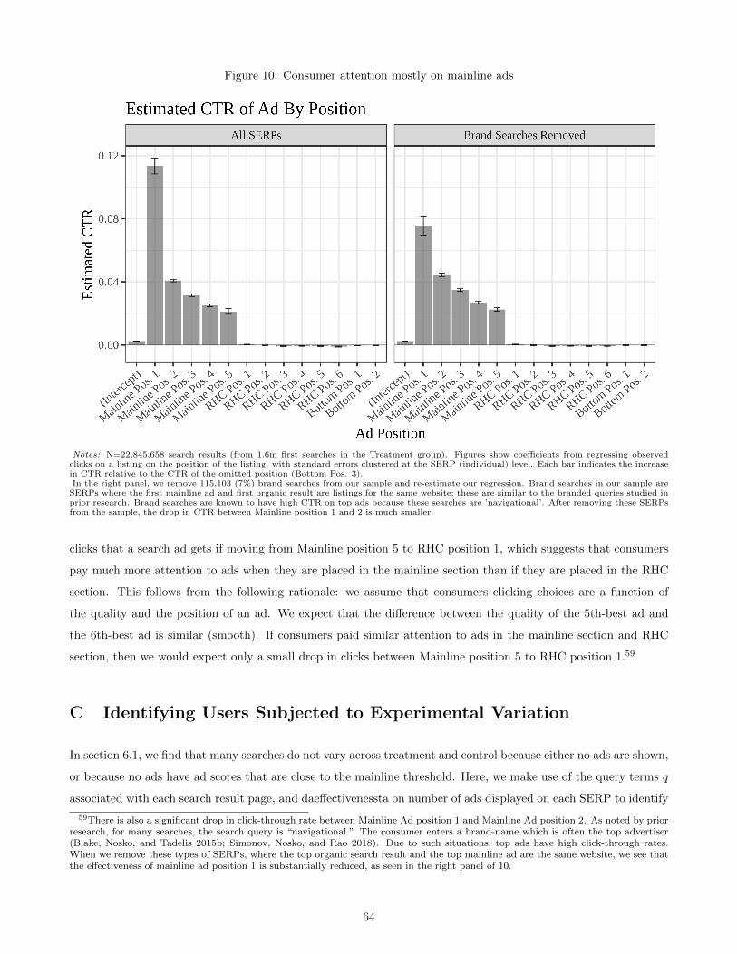
Figure 10: Consumer attention mostly on mainline ads

Notes: N=22,845,658 search results (from 1.6m first searches in the Treatment group). Figures show coefficients from regressing observedclicks on a listing on the position of the listing, with standard errors clustered at the SERP (individual) level. Each bar indicates the increasein CTR relative to the CTR of the omitted position (Bottom Pos. 3).In the right panel, we remove 115,103 (7%) brand searches from our sample and re-estimate our regression. Brand searches in our sample are

SERPs where the first mainline ad and first organic result are listings for the same website; these are similar to the branded queries studied inprior research. Brand searches are known to have high CTR on top ads because these searches are ’navigational’. After removing these SERPsfrom the sample, the drop in CTR between Mainline position 1 and 2 is much smaller.

clicks that a search ad gets if moving from Mainline position 5 to RHC position 1, which suggests that consumers

pay much more attention to ads when they are placed in the mainline section than if they are placed in the RHC

section. This follows from the following rationale: we assume that consumers clicking choices are a function of

the quality and the position of an ad. We expect that the difference between the quality of the 5th-best ad and

the 6th-best ad is similar (smooth). If consumers paid similar attention to ads in the mainline section and RHC

section, then we would expect only a small drop in clicks between Mainline position 5 to RHC position 1.59

C Identifying Users Subjected to Experimental Variation

In section 6.1, we find that many searches do not vary across treatment and control because either no ads are shown,

or because no ads have ad scores that are close to the mainline threshold. Here, we make use of the query terms q

associated with each search result page, and daeffectivenessta on number of ads displayed on each SERP to identify

59There is also a significant drop in click-through rate between Mainline Ad position 1 and Mainline Ad position 2. As noted by priorresearch, for many searches, the search query is “navigational.” The consumer enters a brand-name which is often the top advertiser(Blake, Nosko, and Tadelis 2015b; Simonov, Nosko, and Rao 2018). Due to such situations, top ads have high click-through rates.When we remove these types of SERPs, where the top organic search result and the top mainline ad are the same website, we see thatthe effectiveness of mainline ad position 1 is substantially reduced, as seen in the right panel of 10.

64

which users actually experience the experimental variation. We use this identification for making comparisons in

section 7.2.

Let A(qi) be the number of mainline ads returned by the search engine when a user i submits the query terms qi

to the search engine. Then, if the user is assigned to the Treatment group, he see AT (qi) and if he is assigned to

the Control group, he sees AC(qi). Since i is assigned randomly to treatment or control, we can test if a user who

searched for q would have seen different number of ads in the Treatment or Control group by testing the hypothesis

H0 : AT (q) ≥ AC(q) for every q in our sample.

We run this test for any q that was searched more than 5 times by users in their first search, in both Treatment and

Control groups. We run Welch’s t-test with the unequal variances assumption and count a query q as manipulated

if it is significant (one-sided) at α = .1. We identify 2,298 queries that are likely to have been manipulated, and

these queries are associated with 345,310 first searches.

Note that while this approach allows us to identify query terms that most likely would have returned manipulated

search results, it does not identify all of the queries that were manipulated. We are unable to identify all of the

manipulated queries because many query terms are seen only once (as discussed in section 5.1).

After identifying queries that were likely to have been manipulated, we label users who saw manipulated queries

in their first search as manipulated users (i.e., DManipulatedUser = 1). In Table 3, we showed that these users are

balanced between groups. We find that 10.5% of our sample were likely to have been affected by the experimental

treatment in their first search.

D Quantile Treatment Effects

Tables 16 - 19, and Figures 11 - 14 provide details on the Quantile Treatment effects referred to in the paper.

E Estimated Revenue Procedure

In this section, we discuss how we estimated the change in search engine’s revenue that was reported in section 7.1.

To construct these estimates, we estimate the revenue associated with every observed click that occured during the

experimental period in both the Treatment and Control groups. This allows us to calculate the impact of increasing

mainline search advertsing on revenue. To measure the impact of increasing mainline search advertising on the

revenue of the search engine, we estimate the revenue associated with consumer behavior in the High and Low Ad

conditions of our experiment and calculate the difference in revenue over the duration of the experiment. Ideally,

we would use the actual prices determined in the search engine’s auctions, but we did not have access to this from

our data partner. We rely, instead, on industry estimates of the price-per-click from Google Keyword Planner. We

outline our procedure below.

65

Table 16: Quantile Treatment Effects for Number of Sessions

(a) Total Number of Sessions, Full Sample

Quantile (s) Quantile in Control* Change* (τs) Rel. Change p-value** : H0 : τs < 0

50 1.00 0.00 0.0% <.00175 1.00 0.00 0.0% <.00190 3.00 0.00 0.0% <.00195 6.95 0.04 0.5% 0.008

99.5 49.46 0.84 1.7% 0.018

(b) Total Number of Sessions, subset where DManipulatedUser = 1

Quantile (s) Quantile in Control* Change* (τs) Rel. Change p-value** : H0 : τs < 0

50 1.00 0.00 0.0% <.00175 2.00 0.00 0.0% <.00190 5.00 0.00 0.0% <.00195 10.00 0.14 1.4% <.001

99.5 72.69 4.87 6.7% 0.021

Notes: Tables show the quantile treatment effect (QTE) on TotalSessions at selected quantiles. We present results for (a) the fullsample (N=3,298,086 users) and (b) a subset of users who were exposed to the experimental treatment in their first search (N=345,310users). Details on identifying the subset can be found in Appendix C; more comprehensive QTEs can be found in Appendix D.

*We construct estimates from 10,000 bootstrap samples. We report the average level of the quantile in the control group from our 10,000bootstrap samples, i.e., ¯QY (0)(s), and, following the approach in Athey and Imbens (2017), we estimate the quantile treatment effect τsusing the mean of the bootstrapped QTEs.

**This is the one-sided p-value, testing the null that the quantile treatment effect is negative, i.e. τs < 0 change.

Table 17: Quantile Treatment Effects on Ad Clicks

(a) Ad Clicks, Full Sample

Quantile (s) Quantile in Control* Change* (τs) Rel. Change p-value** : H0 : τs < 0

50 0.00 0.00 0.0% <.00175 0.00 0.00 0.0% <.00190 1.00 0.00 0.0% <.00195 2.00 0.00 0.0% <.001

99.5 19.93 1.07 5.4% <.001

(b) Ad Clicks, subset where DManipulatedUser = 1

Quantile (s) Quantile in Control* Change* (τs) Rel. Change p-value** : H0 : τs < 0

50 0.00 0.00 0.0% <.00175 0.00 0.00 0.0% <.00190 2.00 0.00 0.0% <.00195 4.00 0.01 0.2% <.001

99.5 29.35 4.27 14.5% <.001

Notes: Tables show the quantile treatment effect (QTE) on AdClicks at selected quantiles. We present results for (a) the full sample(N=3,298,086 users) and (b) a subset of users who were exposed to the experimental treatment in their first search (N=345,310 users).Details on identifying the subset can be found in Appendix C; more comprehensive QTEs can be found in Appendix D.

*We construct estimates from 10,000 bootstrap samples. We report the average level of the quantile in the control group from our 10,000bootstrap samples, i.e., ¯QY (0)(s), and, following the approach in Athey and Imbens (2017), we estimate the quantile treatment effect τsusing the mean of the bootstrapped QTEs.

**This is the one-sided p-value, testing the null that the quantile treatment effect is negative, i.e. τs < 0 change.

66

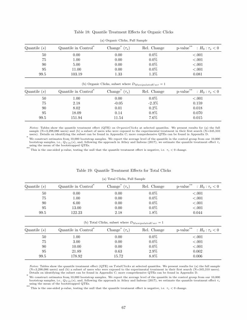
Table 18: Quantile Treatment Effects for Organic Clicks

(a) Organic Clicks, Full Sample

Quantile (s) Quantile in Control* Change* (τs) Rel. Change p-value** : H0 : τs < 0

50 0.00 0.00 0.0% <.00175 1.00 0.00 0.0% <.00190 5.00 0.00 0.0% <.00195 11.00 0.00 0.0% <.001

99.5 103.19 1.33 1.3% 0.081

(b) Organic Clicks, subset where DManipulatedUser = 1

Quantile (s) Quantile in Control* Change* (τs) Rel. Change p-value** : H0 : τs < 0

50 1.00 0.00 0.0% <.00175 2.18 -0.05 -2.3% 0.15990 8.02 0.01 0.2% 0.01895 18.09 0.14 0.8% 0.070

99.5 151.94 11.54 7.6% 0.015

Notes: Tables show the quantile treatment effect (QTE) on OrganicClicks at selected quantiles. We present results for (a) the fullsample (N=3,298,086 users) and (b) a subset of users who were exposed to the experimental treatment in their first search (N=345,310users). Details on identifying the subset can be found in Appendix C; more comprehensive QTEs can be found in Appendix D.

*We construct estimates from 10,000 bootstrap samples. We report the average level of the quantile in the control group from our 10,000bootstrap samples, i.e., ¯QY (0)(s), and, following the approach in Athey and Imbens (2017), we estimate the quantile treatment effect τsusing the mean of the bootstrapped QTEs.

**This is the one-sided p-value, testing the null that the quantile treatment effect is negative, i.e. τs < 0 change.

Table 19: Quantile Treatment Effects for Total Clicks

(a) Total Clicks, Full Sample

Quantile (s) Quantile in Control* Change* (τs) Rel. Change p-value** : H0 : τs < 0

50 0.00 0.00 0.0% <.00175 1.00 0.00 0.0% <.00190 6.00 0.00 0.0% <.00195 13.00 0.00 0.0% <.001

99.5 122.23 2.18 1.8% 0.044

(b) Total Clicks, subset where DManipulatedUser = 1

Quantile (s) Quantile in Control* Change* (τs) Rel. Change p-value** : H0 : τs < 0

50 1.00 0.00 0.0% <.00175 3.00 0.00 0.0% <.00190 10.00 0.00 0.0% <.00195 21.89 0.63 2.9% 0.002

99.5 178.92 15.72 8.8% 0.006

Notes: Tables show the quantile treatment effect (QTE) on TotalClicks at selected quantiles. We present results for (a) the full sample(N=3,298,086 users) and (b) a subset of users who were exposed to the experimental treatment in their first search (N=345,310 users).Details on identifying the subset can be found in Appendix C; more comprehensive QTEs can be found in Appendix D.

*We construct estimates from 10,000 bootstrap samples. We report the average level of the quantile in the control group from our 10,000bootstrap samples, i.e., ¯QY (0)(s), and, following the approach in Athey and Imbens (2017), we estimate the quantile treatment effect τsusing the mean of the bootstrapped QTEs.

**This is the one-sided p-value, testing the null that the quantile treatment effect is negative, i.e. τs < 0 change.

67

Figure 11: Quantile Treatment Effects on Total Visits and Total Sessions

(a) (b)

(c) (d)

Notes: N=3,298,086 users. Figures show the effect of the experimental treatment on the distribution of total visits (plots (a) and (b)) andtotal sessions (plots (c) and (d)). The figures show the average quantile treatment effect τq at percentile q based on 10,000 bootstraps.The effect is in the higher end of the distribution, so we truncate the plots to display the quantile treatment effects for q ∈[60, 99]. Thefigures on the left (plots (a) and (c)) are based on the full sample of users while the figures on the right (plots (b) and (c)) are estimatedusing only users who in their first experimental search typed in a query on which the experimental manipulation took place as described insectionC.

68

Figure 12: Quantile Treatment Effects on Ad Clicks and Organic Clicks

(a) (b)

(c) (d)

Notes: N=3,298,086 users. Figures show the effect of the experimental treatment on the distribution of ad clicks (plots (a) and (b)) andorganic clicks (plots (c) and (d)). The figures show the average quantile treatment effect τq at percentile q based on 10,000 bootstraps.The effect is in the higher end of the distribution, so we truncate the plots to display the quantile treatment effects for q ∈[60, 99]. Thefigures on the left (plots (a) and (c)) are based on the full sample of users while the figures on the right are estimated using only users whoare know to have seen the experimental treatment (plots (b) and (d)) as described in sectionC.

69

Figure 13: Quantile Treatment Effects on Total Clicks

(a) (b)

Notes: N=3,298,086 users. Figure shows the effect of the experimental treatment on the distribution of total clicks. The figures show theaverage quantile treatment effect τq at percentile q based on 10,000 bootstraps. The effect is in the higher end of the distribution, so wetruncate the plots to display the quantile treatment effects for q ∈[60, 99]. The figures on the left plot (a) is based on the full sample ofusers while the right figure (b) is estimated using only users who are known to be affected by the experimental treatment in their firstsearch, as described in sectionC.

E.1 Construction of Estimated Revenue

Let ST be the set of all searches conducted by users assigned to condition T in our experiment (e.g., STreatment is

the set of searches conducted by users in the Treatment condition). Then, s ∈ ST represents a single search.

We denote qs to be the search terms associated with the search s and MainlineClickss and RHCClickss denote

the number of clicks on Mainline and RHC ads, respectively. Then, we could calculate the revenue generated in

condition T as:

RevenueT =∑s∈ST

MainlineClickss × PPCMainline(qs) +RHCClickss × PPCRHC(qs) (38)

where PPCMainline(qs) and PPCRHC(qs) are the prices paid by advertisers60 to the search engine for clicks on

Mainline and RHC search ads when users searched for query terms qs. Since we do not have the actual prices,

however, we must gather price data from another source.

E.2 Gathering Price Data from Google Keyword Planner

Google Keyword Planner (GKP) is a tool offered by Google to help marketing practitioners plan their search

advertising campaigns. GKP provides estimates the cost of running a search advertising campaign that targets

60In reality, prices are generated at auction time and are position-specific. We adopt the formulation in (38) for convenience. Notethat, for example, PPCMainline for some query qs produce accurate estimates of overall revenue if PPCMainline was the position-weighted average of observed prices for all mainline positions.

70

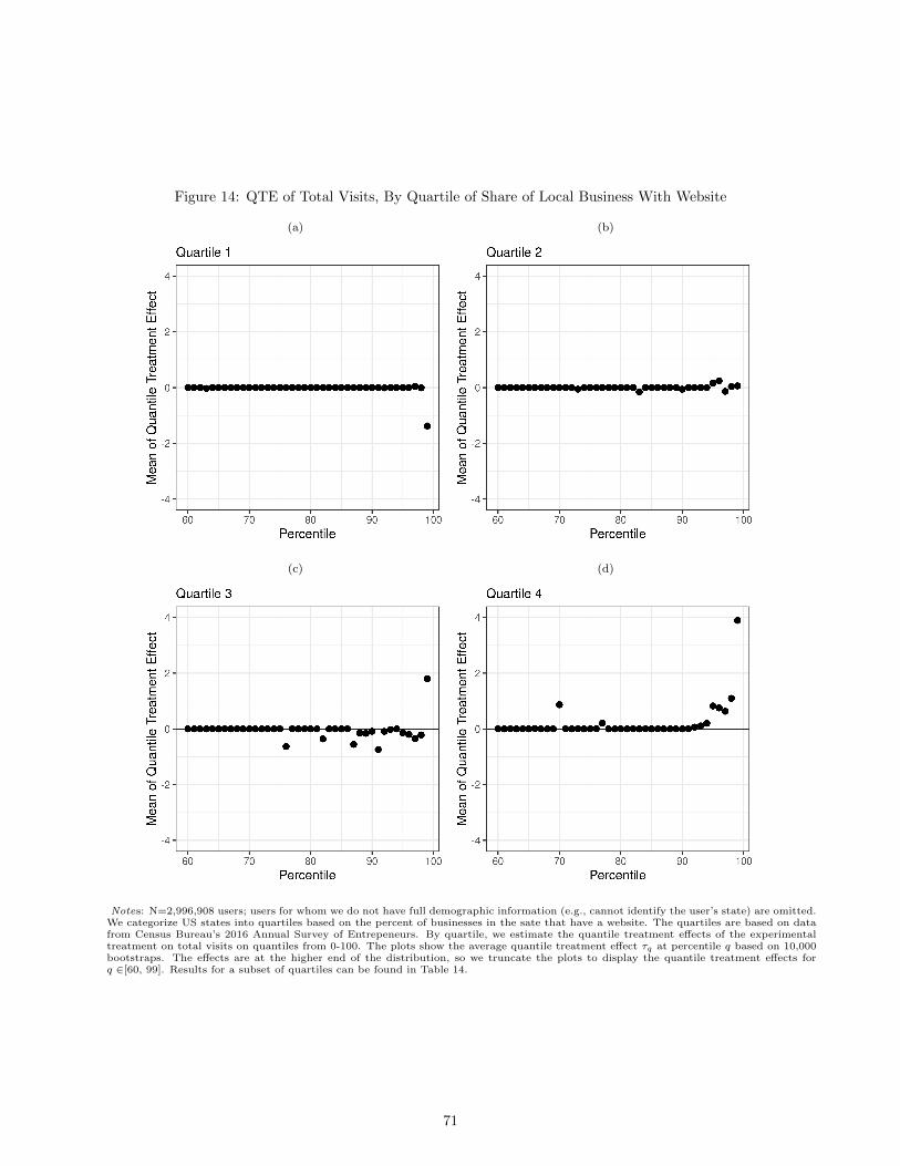
Figure 14: QTE of Total Visits, By Quartile of Share of Local Business With Website

(a) (b)

(c) (d)

Notes: N=2,996,908 users; users for whom we do not have full demographic information (e.g., cannot identify the user’s state) are omitted.We categorize US states into quartiles based on the percent of businesses in the sate that have a website. The quartiles are based on datafrom Census Bureau’s 2016 Annual Survey of Entrepeneurs. By quartile, we estimate the quantile treatment effects of the experimentaltreatment on total visits on quantiles from 0-100. The plots show the average quantile treatment effect τq at percentile q based on 10,000bootstraps. The effects are at the higher end of the distribution, so we truncate the plots to display the quantile treatment effects forq ∈[60, 99]. Results for a subset of quartiles can be found in Table 14.

71

specific query terms (’keywords’) over a certain time period. These estimates are generated by GKP based on the

prices realized historically in search auctions conducted on Google.

We make use of this tool to gather, for all of the observed query terms q, an estimate of the price-per-click paid

to the search engine by advertisers when consumers click on a search ad. Specifically, GKP aggregates the prices

paid by advertisers over the 12 months when consumers searched for the query terms q and reports the 20th (“Top

of page bid - low range”) and 80th (“Top of page bid - high range”) percentile of prices. We gathered data from

GKP for all of the relevant query terms q in November 2018 and use these as our estimates of price-per-click for

q. This data allows us to describe high and low ranges of PPCs through the PPClow(q) and PPChigh(q), which

correspond to the 20th and 80th percentile prices respectively.

For search terms q which GKP returns no PPC data, we set the PPC to $0.00 as this indicates to us that there is

little competition on the query terms q. We match roughly 60% of all of the ad clicks seen on the search engine.

E.3 Combining Estimates

We calculate our initial estimate using both PPChigh(q) and PPClow(q). We assume that the search engine receives

the 80th percentile PPC for Mainline Ad clicks and the 20th percentile PPC for RHC clicks.

HighEstimatedRevenueT =∑s∈ST

MainlineClickss × PPChigh(qs) +RHCClickss × PPClow(qs) (39)

alternatively, we can lower bound the impact by assuming that our search engine is only able to receive payments

similar to the low range of PPCs for Mainline Ad clicks:

LowEstimatedRevenueT =∑s∈ST

MainlineClickss × PPClow(qs) +RHCClickss × PPClow(qs) (40)

These estimates are reported in Table (7).

72