1 Cographsi Robert Haas 1. Introduction This article ... - arXiv

1

Cographsi

Robert Haas

1. Introduction

This article introduces the theory of cographs, combinatorial structures that both dualize

and generalize ordinary graphs; they promise as rich a range as graph theory itself of applications

inside and outside mathematics. Their double origin produces two equivalent definitions. For the

first, note that a graph may be defined abstractly as a function (a primitive boundary operator)

G: E → P(2) that associates to each element of an abstract set E (“edges”) an (unordered) pair of

distinct elements from the abstract set P (“points”) called the element’s “endpoints.” Dualizing:

Definition 1.1. A cograph is a set function C: P(2) → E, where elements of P are “points,” elements

of E are “edges,” and P(2) is (unordered) pairs of distinct points of P.

Representing the cograph C by ordinary points, and lines between each pair of points, yields the

equivalent second definition:

Definition 1.2. A cograph is a complete graph with colored lines.

Here the complete graph Kn is the graph on n points where each pair is joined by a line. In keeping

with the desired abstract combinatorial nature of cographs, the second definition actually involves

classes of graphs equivalent under position or color labeling: In the cographs with three points, for

example, no distinction will be made between the triangle having a red lower line and blue right

and left sides, and the same triangle rotated to put its red line at the right; or from the triangle with

one yellow and two green lines; or from the one with one blue and two red lines.

Remark. Note that it is not required that lines incident at a point have different colors. This type

of constraint, common in graph coloring theory, can introduce considerable combinatorial

complexity (e.g. Haas [10]), and examples below show it does not hold in some quite natural

classes of cographs.

Figure 1.1 shows the three cographs on 3 points, representing the colors by patternings--

solid, dashed, or dotted--of the edges; “Type” classifies the cographs by the number of copies of

each edge.

Type 3 Type 2+1 Type 1+1+1

Fig. 1.1. The three cographs on three points.

2

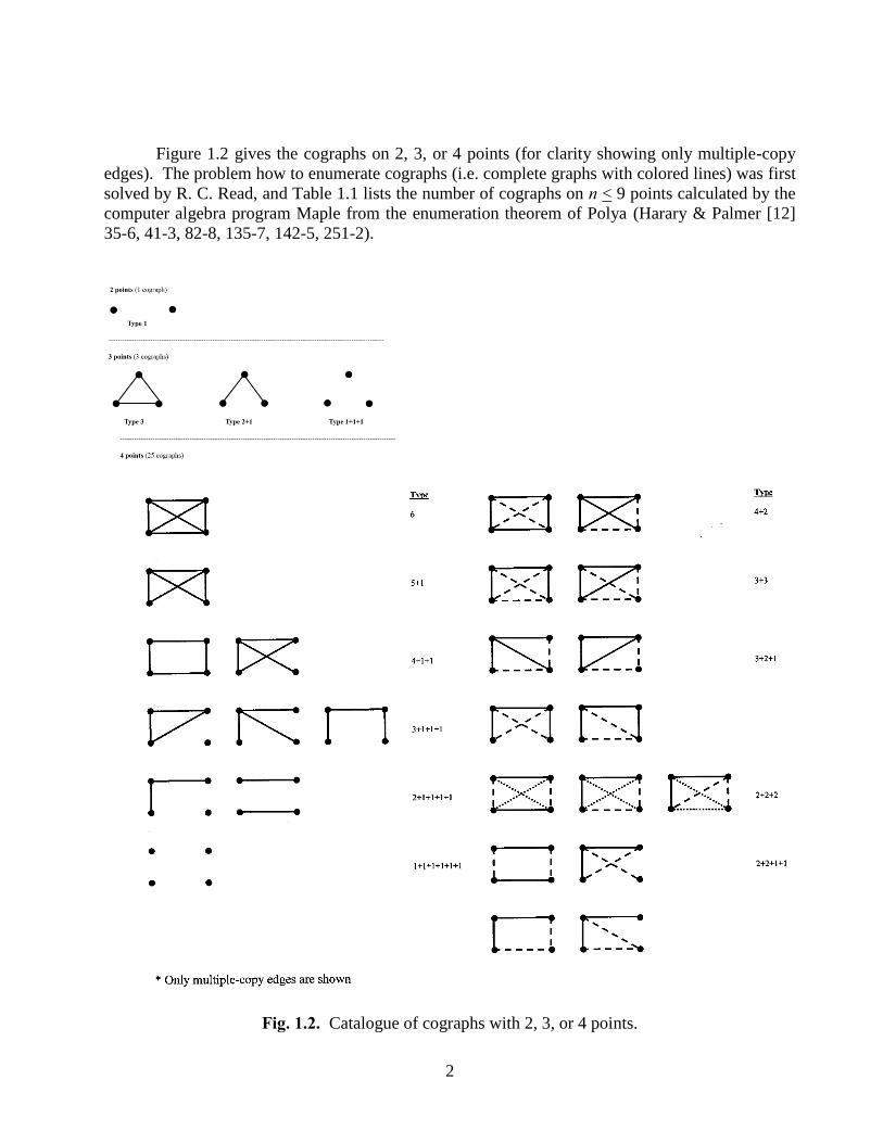
Figure 1.2 gives the cographs on 2, 3, or 4 points (for clarity showing only multiple-copy

edges). The problem how to enumerate cographs (i.e. complete graphs with colored lines) was first

solved by R. C. Read, and Table 1.1 lists the number of cographs on n < 9 points calculated by the

computer algebra program Maple from the enumeration theorem of Polya (Harary & Palmer [12]

35-6, 41-3, 82-8, 135-7, 142-5, 251-2).

Fig. 1.2. Catalogue of cographs with 2, 3, or 4 points.

3

Table 1.1. Number of Cographs on n Points

Points (n) Cographs 2 1

3 3

4 25

5 1299

6 1.97 x 106

7 9.43 x 1010

8 1.53 x 1017

9 1.05 x 1025

Appreciation how cographs generalize other combinatorial structures comes from

considering the ones with just a few edges. Cographs with a single edge coincide with complete

graphs Kn (or equivalently with their complements Kn having n points and no lines). Viewing a

cograph with two edges as being a graph with black and (invisible) white lines shows how it

coincides with an ordinary graph (or, again, the complement). Any cograph thus naturally breaks

up into a line-disjoint union of graphs, one for each color, on the same set of points. And, as

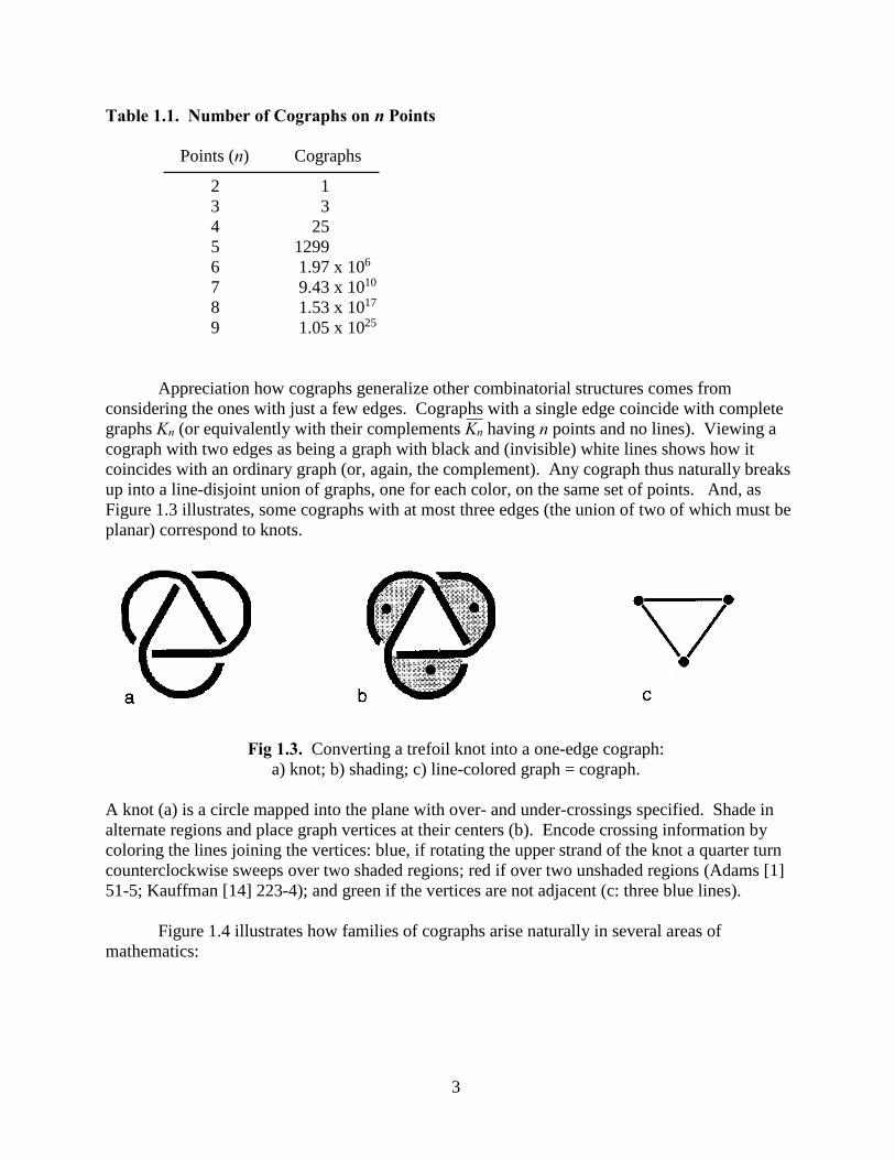
Figure 1.3 illustrates, some cographs with at most three edges (the union of two of which must be

planar) correspond to knots.

Fig 1.3. Converting a trefoil knot into a one-edge cograph:

a) knot; b) shading; c) line-colored graph = cograph.

A knot (a) is a circle mapped into the plane with over- and under-crossings specified. Shade in

alternate regions and place graph vertices at their centers (b). Encode crossing information by

coloring the lines joining the vertices: blue, if rotating the upper strand of the knot a quarter turn

counterclockwise sweeps over two shaded regions; red if over two unshaded regions (Adams [1]

51-5; Kauffman [14] 223-4); and green if the vertices are not adjacent (c: three blue lines).

Figure 1.4 illustrates how families of cographs arise naturally in several areas of

mathematics:

4

{1,2,3} {1,2} 1 2 1 2

{1,2,4} {1,3} 4 3 0 3

a) Intersection cograph b) Sum cograph c) Distance cograph

Fig. 1.4. Some simple mathematical cographs.

In an intersection cograph (a) the points are sets, and the edge C(P,Q) joining points P and Q is their

intersection P ∩ Q. In algebraic cographs the points are elements of an algebraic structure, and

edges the corresponding algebraic product; thus in sum cograph (b) the points are integers, with

C(P,Q) = P + Q. Metric structures are yet another source of cographs: in the distance cograph (c)

the points are real numbers, with C(P,Q) = |P-Q|.

One theme in this study will be to investigate which cographs can arise in each of these

various ways. Figure 1.5 illustrates some configurations that are forbidden to occur:

P Q P Q R P R S Q R

a) In an intersection cograph b) In a sum cograph over c) In a distance cograph over

an abelian group the real numbers

Fig. 1.5. Forbidden configurations.

For in (a), a ≠b, yet a = a ∩ a = (P ∩ Q) ∩ (R ∩ S) = (P ∩ R) ∩ (Q ∩ S) = b ∩ b = b; in (b), P ≠ R,

yet P+Q = C(P,Q) = C(Q,R) = Q+R implies P = R; and in (c), relabeling points, if necessary, to

make P < Q < R, C(P,R) = R-P = (R-Q) + (Q-P) = C(Q,R) + C(P,Q) = 2 C(P,R), a contradiction.

Remarks. 1.1) Other variants: One might also define a “union cograph” on sets, with C(P,Q) =

P Q; but taking complements and applying DeMorgan’s laws, the same cograph may be

obtained as an intersection cograph. “Number theoretic cographs,” with C(P,Q) being the gcd or

lcm of numbers P and Q, are likewise just variants of intersection cographs.

1.2) Intersection cographs as algebraic: An intersection cograph is equivalent to an

algebraic cograph of the form Z2 ⨁ ... ⨁ Z2 indexed by the union of the sets of the cograph. For

simply replace each point or edge S by the “characteristic function” χS that is 1 exclusively on

coordinates in S, and set intersections then correspond to products in the ring.

{1,2}

{1}

{1,3}

3

5

4

6

7

1

3

2

a

b

5

1.3) Potential applications: This initial article must focus on the mathematics of cographs;

but intersection cographs, especially, promise to be useful for modeling real-world phenomena.

One might model, for instance, the people participating in social or political interactions as each

one equivalent to the set of his own “interests,” and describe a process like negotiation as a search

through cographs for maximal overlap. Table 1.1, showing the vast numbers of possible cographs

(i.e. configurations, alignments, coalitions) on even a few points, might give insight why reaching

consensus can sometimes be so difficult. A similar viewpoint appears in branches of philosophy

that regard every object as underlying “substance” bearing the set of its “accidents.” Another class

of applications might let cograph edges represent forces between the points: a crystal, atoms held

together by electrostatic forces between each pair; a galaxy, stars held by pairwise gravitational

attraction; a poem, words each linked to many others by sound or sense. (See §4.2 for further

applications to aesthetics.)

As a first theorem about cographs, one proves that they may be represented in several ways:

Theorem 1.1. Every cograph may be represented as 1) a “fat” intersection cograph. Every finite

cograph may also be represented as 2a) an inner product cograph, 2b) a polynomial cograph, and

3) a sufficiently high-dimensional geometric cograph.

Proof. 1) Let P and S be collections of sets, where S is closed under intersections and contains

U = P . Define a fat intersection cograph F to have points P, where the edge F(P,Q) is the

smallest set in S containing P ∩ Q.

Fig. 1.6. Example of a fat intersection cograph. {a,c} {a,d} Let S = {∅, {a,b}, {c,d}, {a,b,c,d}}.

(Note that this contains the configuration of

Figure 1.5a, hence is not an intersection cograph.) {b,c} {b,d}

Given then an abstract cograph C, first make the copies of each edge distinguishable by relabeling

C(P,Q) = e as C’(P,Q) = e{P,Q}, and then label each point P with the set P* = Po {e{P,Q}}.

Then, for all P and Q, P* ∩ Q* is precisely C ’(P,Q). Define U = P*, and define the set S as:

S = {∅, U} {e{P,Q}: e{P,Q} is a relabeled copy of e}

Edges then belong to the same set in S ~ {∅, U} if and only if they originated from multiple copies

in C, and thus C is equivalent to the fat intersection cograph with points P* and list S.

2a) The n-point abstract cograph C will be represented by an (n-1)-dimensional inner

product cograph I--its points from a real inner product space X, the edge between two points

defined as their inner (dot) product, I(P,Q) = (P,Q)--making an arbitrary choice of distinct real

numbers for the edges. Thus the goal is to represent each point Pi (1<i<n) of C by a point

(pi1,pi2,...,pi(n-1)) in I. As an initial labeling, let P1 be (1,0,...,0), and let pi1 = C(P1,Pi) for i = 2,3,...,n.

Proceeding inductively, once pij has been defined for i,j < k, let pkk = 1, pki = 0 for i>k, and for i<k

let pik = C(Pi,Pk) - ∑ pijpkj. From this construction, the edge label C(Pi,Pj) coincides with the inner

product. P1,P2,...,Pn-1 have distinct labels (since pij = 1 when i = j and 0 when i<j), but not

necessarily Pn. To guarantee it distinct the initial labeling must be modified. At the cost of

increasing the dimension, one can simply add an nth coordinate, 0 for P1,P2,...,Pn-1 and 1 for Pn.

P P

{a,b}

{c,d}

∅

QC

P C

e C

j=1

k-1

6

Otherwise, one modifies the initial labeling stepwise: find the lowest index i where Pi coincides

with Pn, and change pii from 1 to 2, and pik to half its value for k>i; then repeat inductively to

eliminate any introduced new coincidences.

Remark. The bound on the dimension is the best possible: It can be shown that the cograph with

n points (n > 3) and a single edge cannot be represented by an inner product cograph of dimension

n-2.

2b) The n-point abstract cograph C will be represented by a polynomial cograph P--its

points from Z (or Zm), the edge P(P,Q) defined to equal f(P,Q) where f is a symmetric polynomial

in two variables--labeling the points of C by the integers 1,2,...,n, and its edges by arbitrarily

chosen distinct positive integers. Define first a family of elementary symmetric polynomials fij,

1<i<j<n, by fij(x,y) = ∏ [(x-s)2 + (y-t)2].[(x-t)2 + (y-s)2]; thus fij(i,j) = fij(j,i) ≠ 0, but fij(x,y) = 0

otherwise. A symmetric interpolatory polynomial f satisfying f(P,Q) = C(P,Q) for all the chosen

values of C(P,Q) will then be an appropriate linear combination, with rational coefficients, of the

fij’s. Multiplying f by a constant to clear the denominator will not change the cograph, which is

thus over Z (or, since finite, in Zm for sufficiently large m).

3) The goal is to represent the n-point abstract cograph C by a geometric cograph G--points

from Rn-1, Euclidean distances for edges. The cograph with just one edge (of length 1) is given by

the points (1/√2, 0,0,...,0), (0, 1/√2,0,...,0),...,(0,0,0,...,0, 1/√2), and (c,c,c,...,c), where c =

(1+ 1/√(n+1))/(n/√2). To obtain a cograph with more edges one adjusts edge lengths in this figure:

any side independently can be expanded slightly by moving an endpoint in a way that changes the

angles but not the lengths of the other sides. The sole “geometric” constrant is that subpolyhedra

remain nondegenerate, i.e. keep nonzero volume, and these volumes can be expressed by

determinants (Borsuk [5] 116-120) which are continuous functions of the coordinates, hence

remain bounded away from zero within small neighborhoods. Hence for a sufficiently large

integer K one may convert the starting cograph to an arbitrary one with m edges, where edge i has

length 1+i/K, for i = 1,2,...,m. Since scaling the figure up by a factor of K does not change the

cograph, this proof also shows that one can realize an arbitrary finite cograph by a geometric

cograph with edges of integer lengths.

Remarks. The constraint on dimensions is the best possible: one cannot realize a three-point

cograph with one edge--an equilateral triangle--in R1. Note also that geometric representation is

not always possible with rational or integer points--for instance, there is no equilateral triangle with

all three vertices rational in R2. ■

Theorem 1.1 seeks concrete terms like sets for both points and edges to produce a given

abstract cograph--the cograph representation problem, that in general seems quite difficult. To

conclude this section, here are some results for the easier situation in which the cograph edges are

“prelabeled,” and the problem is only to find the points.

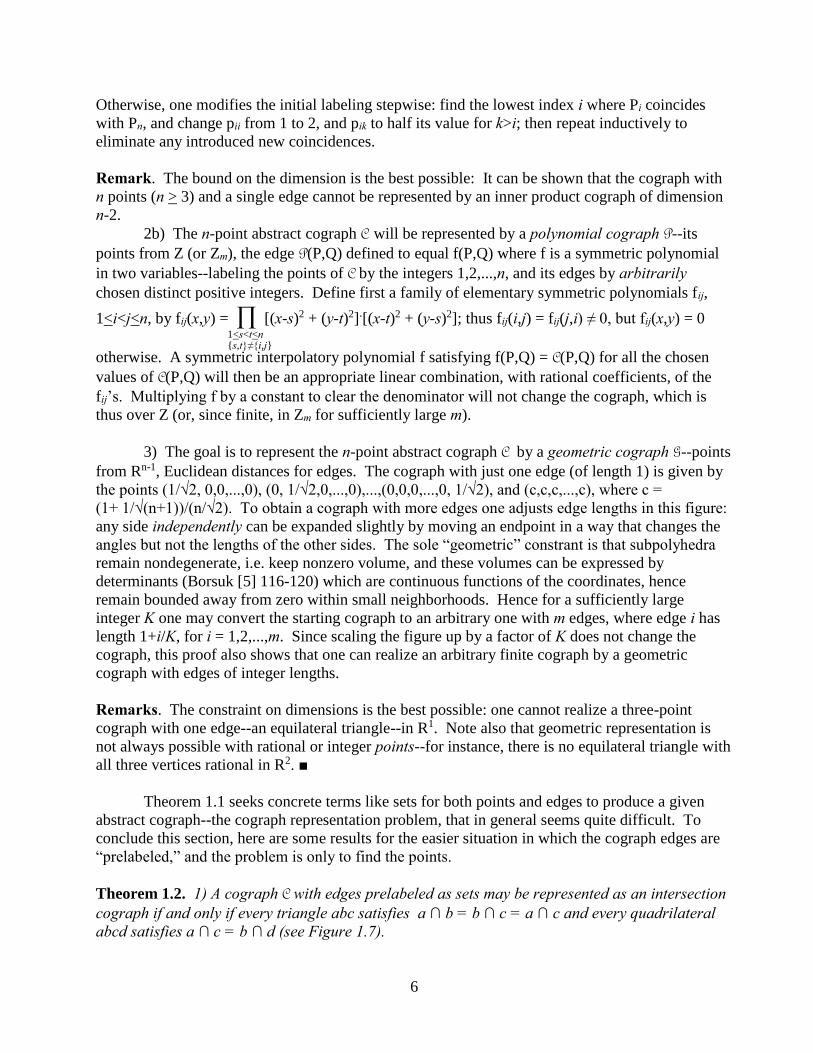
Theorem 1.2. 1) A cograph C with edges prelabeled as sets may be represented as an intersection

cograph if and only if every triangle abc satisfies a ∩ b = b ∩ c = a ∩ c and every quadrilateral

abcd satisfies a ∩ c = b ∩ d (see Figure 1.7).

1<s<t<n {s,t}≠{i,j}

7

a a

P Q P Q

c b d b

R S R

c

Fig. 1.7. A triangle and a quadrilateral.

Each point P may then be labeled with the set P’ = {Po} C(P,Q) , where Po is a unique “point

name” (i.e. P’ ∩ Q’ = C(P, Q) for all P and Q in C).

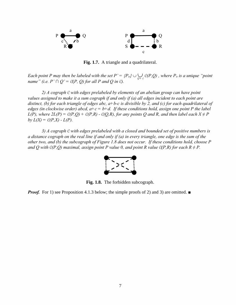
2) A cograph C with edges prelabeled by elements of an abelian group can have point

values assigned to make it a sum cograph if and only if (a) all edges incident to each point are

distinct, (b) for each triangle of edges abc, a+b-c is divisible by 2, and (c) for each quadrilateral of

edges (in clockwise order) abcd, a+c = b+d. If these conditions hold, assign one point P the label

L(P), where 2L(P) = C(P,Q) + C(P,R) - C(Q,R), for any points Q and R, and then label each X ≠ P

by L(X) = C(P,X) - L(P).

3) A cograph C with edges prelabeled with a closed and bounded set of positive numbers is

a distance cograph on the real line if and only if (a) in every triangle, one edge is the sum of the

other two, and (b) the subcograph of Figure 1.8 does not occur. If these conditions hold, choose P

and Q with C(P,Q) maximal, assign point P value 0, and point R value C(P,R) for each R ≠ P.

Fig. 1.8. The forbidden subcograph.

Proof. For 1) see Proposition 4.1.3 below; the simple proofs of 2) and 3) are omitted. ■

Q

C

Q

C

C

Q C

8

a

c

2.1. Sum cographs: Elementary properties

A sum cograph, as mentioned above, is a cograph having its points and edges in an abelian

group, in which each edge is simply the sum of its endpoints: C(P,Q) = P+Q. In consequence,

Q = C(P,Q) - P, and, inductively, the value of each point in any chain of points and edges is

determined by the initial point P and the alternating sum of the intervening edges, as follows:

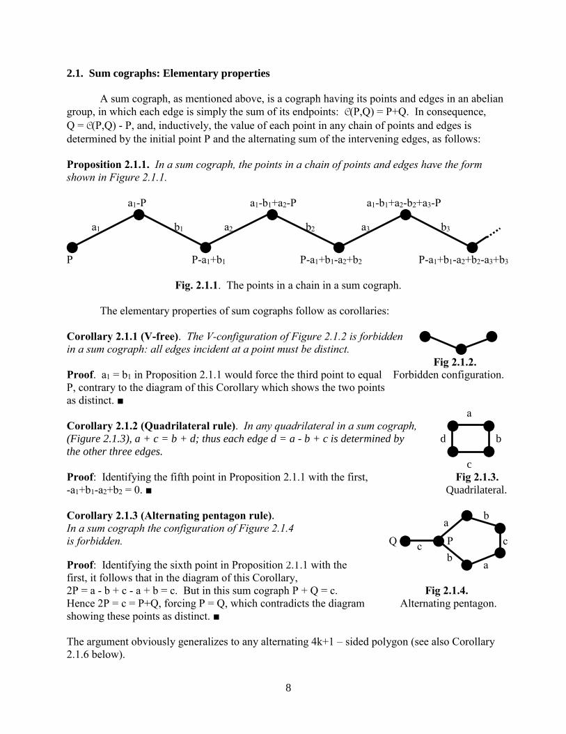
Proposition 2.1.1. In a sum cograph, the points in a chain of points and edges have the form

shown in Figure 2.1.1.

a1-P a1-b1+a2-P a1-b1+a2-b2+a3-P a1 b1 a2 b2 a3 b3

P P-a1+b1 P-a1+b1-a2+b2 P-a1+b1-a2+b2-a3+b3

Fig. 2.1.1. The points in a chain in a sum cograph.

The elementary properties of sum cographs follow as corollaries:

Corollary 2.1.1 (V-free). The V-configuration of Figure 2.1.2 is forbidden

in a sum cograph: all edges incident at a point must be distinct. Fig 2.1.2.

Proof. a1 = b1 in Proposition 2.1.1 would force the third point to equal Forbidden configuration.

P, contrary to the diagram of this Corollary which shows the two points

as distinct. ■

aCorollary 2.1.2 (Quadrilateral rule). In any quadrilateral in a sum cograph, (Figure 2.1.3), a + c = b + d; thus each edge d = a - b + c is determined by d b

the other three edges. c

Proof: Identifying the fifth point in Proposition 2.1.1 with the first, Fig 2.1.3.

-a1+b1-a2+b2 = 0. ■ Quadrilateral.

Corollary 2.1.3 (Alternating pentagon rule). b

In a sum cograph the configuration of Figure 2.1.4

is forbidden. Q P c Proof: Identifying the sixth point in Proposition 2.1.1 with the a

first, it follows that in the diagram of this Corollary,

2P = a - b + c - a + b = c. But in this sum cograph P + Q = c. Fig 2.1.4.

Hence 2P = c = P+Q, forcing P = Q, which contradicts the diagram Alternating pentagon.

showing these points as distinct. ■

The argument obviously generalizes to any alternating 4k+1 – sided polygon (see also Corollary

2.1.6 below).

c

a

b

9

Corollary 2.1.4 (Forced hexagon). In a sum cograph, the configuration of Figure 2.1.5, part (a),

forces that of part (b).

(a) (b)

Fig. 2.1.5. Configuration a forces configuration b.

Proof: The central vertical edge of the hexagon bisects it into two equal three-sided figures, and

Corollary 2.1.2, the quadrilateral rule, then forces the two vertical side edges of the hexagon to be

equal. ■

Corollary 2.1.4 and Corollary 2.1.1 together yield, incidentally, an alternate proof for

Corollary 2.1.3.

Corollary 2.1.5 (Alternating n-cycle). If a sum cograph contains an alternating cycle of (even)

length n, its group must have an element with n/2-torsion.

Proof. In Proposition 2.1.1, denote a1 = a2 = ... = an/2 = a and b1 = b2 = ... = bn/2 = b. Then the

n+1st point is P - (n/2)a + (n/2)b. That the chain closes to a cycle means this point is again P, so

(n/2)(b-a) = 0, and b-a has n/2-torsion. ■

Corollary 2.1.6 (2-Torsion). If a sum cograph contains either two identical odd cycles, or the

configuration of Figure 2.1.6b, then its group must have 2-torsion.

P0 Q0 P P4 P1 Q4 Q1 P3 P2 Q3 Q2 Q

(a) (b)

Fig. 2.1.6. Configurations forcing 2-torsion

Proof. We illustrate the proof in the case that the cograph contains two 5-cycles (Figure 2.1.6(a)).

Then 2P0 = (P0 + P1) - (P1 + P2) + (P2 + P3) - (P3 + P4) + (P4 + P0) = e0 - e1 + e2 - e3 +e4 =

(Q0 + Q1) - (Q1 + Q2) + (Q2 + Q3) - (Q3 + Q4) + (Q4 + Q0) = 2Q0, and if the group lacks 2-torsion

then P0 = Q0. Similarly, Pi = Qi for all i, contradicting the assumption that the two cycles are

distinct.

e0

e2

e4

e4

e0

e3

P0

e2

e3

a

o

h

e1

e1

e3

10

In the case of Figure 2.1.6(b), the edge b = C(P,Q) = P + Q splits the figure to two

quadrilaterals, for which the quadrilateral rule, Corollary 2.1.2, implies 2a - h = b = 2o - h, forcing

the contradiction a = o unless the group has 2-torsion. ■

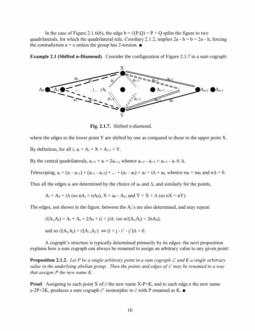
Example 2.1 (Shifted n-Diamond). Consider the configuration of Figure 2.1.7 in a sum cograph:

X

A0 A1 ... Ai Ai+1 ... An-2An-1 Y Fig. 2.1.7. Shifted n-diamond.

where the edges to the lower point Y are shifted by one as compared to those to the upper point X.

By definition, for all i, ai = Ai + X = Ai-1 + Y.

By the central quadrilaterals, ai+2 + ai = 2ai+1, whence ai+2 - ai+1 = ai+1 - ai ≡ Δ.

Telescoping, ai = (ai - ai-1) + (ai-1 - ai-2) + ... + (a1 - a0) + a0 = iΔ + a0, whence nai = na0 and nΔ = 0.

Thus all the edges ai are determined by the choice of a0 and Δ, and similarly for the points,

Ai = A0 + iΔ (so nAi = nA0), X = a0 - A0, and Y = X + Δ (so nX = nY).

The edges, not shown in the figure, between the Ai’s are also determined, and may repeat:

C(Ai,Aj) = Ai + Aj = 2A0 + (i + j)Δ (so nC(Ai,Aj) = 2nA0),

and so C(Ai,Aj) = C(Ai’,Aj’) ⇔ (i + j - i’ - j’)Δ = 0.

A cograph’s structure is typically determined primarily by its edges: the next proposition

explains how a sum cograph can always be renamed to assign an arbitrary value to any given point:

Proposition 2.1.2. Let P be a single arbitrary point in a sum cograph C, and K a single arbitrary

value in the underlying abelian group. Then the points and edges of C may be renamed in a way

that assigns P the new name K.

Proof. Assigning to each point X of C the new name X-P+K, and to each edge e the new name

e-2P+2K, produces a sum cograph C’ isomorphic to C with P renamed as K. ■

a0

ai

ai+1

an-1

an-2

a1

a1

a2

ai+1

ai+2

an-1

a0

11

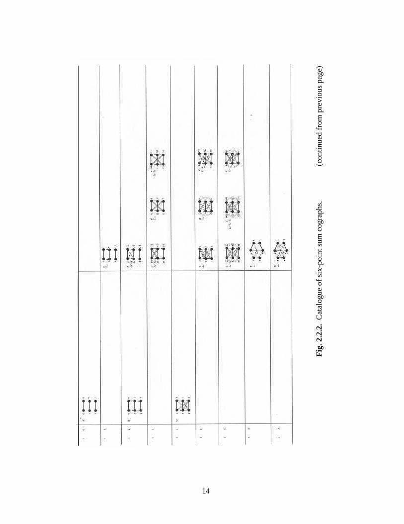
2.2. Sum cographs on six points

The catalogue Figure 2.2.2 below presents the 55 sum cographs on six points (showing only

repeated edges), and Table 2.1 lists their general and particular numerical representations and other

invariants. Since sum cographs on two to five points can naturally be extended to six points by

adding isolated points with high numerical values, the figure and table actually present all sum

cographs on six or fewer points.

The cographs were built up systematically by adding increasing numbers of pairs or triples

of equal edges. Hence the finished figure is complete. A complementary concern is whether the

process might have left duplicates, arriving at the same final structure by distinct paths. But the

numerical invariants in the table, counting number of repeated edges and their degrees at each

point, suffice to prove that these cographs are all distinct.

The construction involved analyzing well over 400 candidate structures. So any tabulation

on more than six points will surely require computer assistance.

The cographs are sorted by number of repeated pairs or triples of edges, and whether they

require torsion elements. Any (finite) sum cograph can, of course, be realized in a sufficiently

large torsion group. But since some simple cograph configurations force torsion (see, e.g.,

Corollaries 2.1.5 and 2.1.6 and Example 2.1 in the preceding section), torsion-free solutions are

likely increasingly rare in large cographs, so seem worthy of special note.

In the table, note that for the point degrees and edge multiplicities only multiple edges are

counted. In the general P,Q,R,… representations, the forms like P+Q-R or 3Q-2P are explicable by

the fact that increasing the value of each variable by 1 yields another valid representation. Thus if

X = Σ aiXi, then X+1 = Σ ai(Xi+1), and by subtraction, Σ ai = 1. Also useful in finding convenient

representations is that fact that if {Xi} is a representation, so is {M-Xi}, for any fixed value M.

Construction of Figure 2.2.2

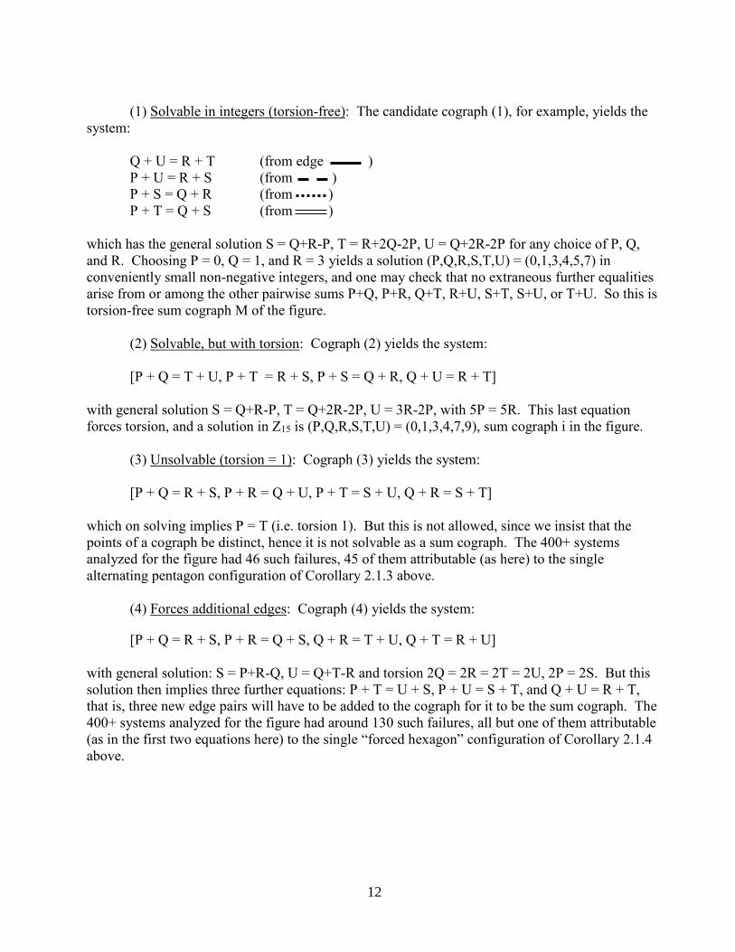
A candidate cograph structure yields a system of linear equations, which can have one of

four possible outcomes when one tries to solve it:

(1) (2) (3) (4)

P S S

U T P Q U T Q R S R P Q R S R T U Q P T U

Solvable in integers Solvable, with torsion Unsolvable Forces additional edges

Figure 2.2.1. Cographs illustrating the four possible outcomes

12

(1) Solvable in integers (torsion-free): The candidate cograph (1), for example, yields the

system:

Q + U = R + T (from edge )

P + U = R + S (from )

P + S = Q + R (from )

P + T = Q + S (from )

which has the general solution S = Q+R-P, T = R+2Q-2P, U = Q+2R-2P for any choice of P, Q,

and R. Choosing P = 0, Q = 1, and R = 3 yields a solution (P,Q,R,S,T,U) = (0,1,3,4,5,7) in

conveniently small non-negative integers, and one may check that no extraneous further equalities

arise from or among the other pairwise sums P+Q, P+R, Q+T, R+U, S+T, S+U, or T+U. So this is

torsion-free sum cograph M of the figure.

(2) Solvable, but with torsion: Cograph (2) yields the system:

[P + Q = T + U, P + T = R + S, P + S = Q + R, Q + U = R + T]

with general solution S = Q+R-P, T = Q+2R-2P, U = 3R-2P, with 5P = 5R. This last equation

forces torsion, and a solution in Z15 is (P,Q,R,S,T,U) = (0,1,3,4,7,9), sum cograph i in the figure.

(3) Unsolvable (torsion = 1): Cograph (3) yields the system:

[P + Q = R + S, P + R = Q + U, P + T = S + U, Q + R = S + T]

which on solving implies P = T (i.e. torsion 1). But this is not allowed, since we insist that the

points of a cograph be distinct, hence it is not solvable as a sum cograph. The 400+ systems

analyzed for the figure had 46 such failures, 45 of them attributable (as here) to the single

alternating pentagon configuration of Corollary 2.1.3 above.

(4) Forces additional edges: Cograph (4) yields the system:

[P + Q = R + S, P + R = Q + S, Q + R = T + U, Q + T = R + U]

with general solution: S = P+R-Q, U = Q+T-R and torsion 2Q = 2R = 2T = 2U, 2P = 2S. But this

solution then implies three further equations: P + T = U + S, P + U = S + T, and Q + U = R + T,

that is, three new edge pairs will have to be added to the cograph for it to be the sum cograph. The

400+ systems analyzed for the figure had around 130 such failures, all but one of them attributable

(as in the first two equations here) to the single “forced hexagon” configuration of Corollary 2.1.4

above.

13

Fig

. 2.2

.2. C

atal

ogue

of

six

-poin

t su

m c

ogra

phs.

(c

onti

nued

nex

t pag

e)

14

Fig

. 2.2

.2.

Cat

alo

gue

of

six

-poin

t su

m c

ogra

phs

(conin

ud f

rom

tin

e

Fig

. 2.2

.2. C

atal

ogue

of

six

-poin

t su

m c

ogra

phs.

(co

nti

nu

ed f

rom

pre

vio

us

pag

e)

15

Tri

ple s

Pai

rs

Co

-

gra ph

N

um

eri

cal G

rou

p

Po

int

de

gre

es

Ed

ge

mu

lti-

plicit

ies

PQ

RS

TU

To

rsio

n

TO

RS

ION

-FR

EE

00

A0 1

2 4

7 1

2Z

0 0

0 0

0 0

0P

QR

ST

U

01

B0 1

2 3

6 1

0Z

0 0

1 1

1 1

2P

QR

P+Q

-RT

U

02

C0 1

2 4

7 8

Z0 1

1 2

2 2

2 2

PQ

2Q

-PS

TQ

+T-P

02

D0 1

2 3

6 9

Z

1 1

1 1

2 2

2 2

PQ

RQ

+R

-PT

Q+R

+T-2

P

03

E0 1

2 3

4 8

Z0 2

2 2

3 3

2 2

2P

Q2Q

-P3Q

-2P

4Q

-3P

U

03

F0 1

2 3

5 8

Z1 1

2 2

3 3

2 2

2

PQ

RQ

+R

-PQ

+2R

-2P

2Q

+3R

-4P

03

G0 1

2 4

6 7

Z1 2

2 2

2 3

2 2

2

PQ

2Q

-PS

2Q

+S

-2P

3Q

+S

-3P

03

H0 1

2 4

5 8

Z1 1

1 3

3 3

2 2

2P

Q2Q

-PS

Q+S

-P2S

-P

03

I0 1

2 3

6 8

Z2 2

2 2

2 2

2 2

2P

QR

Q+R

-PT

R+T-P

04

J0 1

2 3

4 7

Z1 2

3 3

3 4

2 2

2 2

PQ

2Q

-P3Q

-2P

4Q

-3P

7Q

-6P

04

K0 1

2 4

5 7

Z2 2

2 3

3 4

2 2

2 2

PQ

2Q

-P4Q

-3P

5Q

-4P

7Q

-6P

04

L0 1

2 3

5 7

Z2 2

3 3

3 3

2 2

2 2

PQ

RQ

+R

-PQ

+2R

-2P

Q+3R

-3P

04

M0 1

3 4

5 7

Z2 2

3 3

3 3

2 2

2 2

PQ

RQ

+R

-PR

+2Q

-2P

Q+2R

-2P

05

N0 1

2 3

4 6

Z2 3

3 4

4 4

2 2

2 2

2P

Q2Q

-P3Q

-2P

4Q

-3P

6Q

-5P

05

O0 1

2 3

5 6

Z3 3

3 3

4 4

2 2

2 2

2P

Q2Q

-P3Q

-2P

5Q

-4P

6Q

-5P

10

A’

0 1

3 5

7 8

Z1 1

1 1

1 1

3P

QR

SR

+S

-QR

+S

-P

12

B’

0 1

2 4

5 6

Z2 2

2 2

3 3

2 2

3P

Q2Q

-PS

Q+S

-PS

+2Q

-2P

14

C’

0 1

2 3

4 5

Z3 3

4 4

4 4

2 2

2 2

3P

Q2Q

-P3Q

-2P

4Q

-3P

5Q

-4P

Tab

le 2

.1. S

ix-p

oin

t su

m c

ogra

phs:

Rep

rese

nta

tions

and i

nvar

iants

.

(conti

nued

nex

t pag

e)

16

Tri

ple s

Pai

rs

Co

-

gra ph

N

um

eri

cal

Gro

u

p

Po

int

de

gre

es

Ed

ge

mu

lti-

plicit

ies

PQ

RS

TU

To

rsio

n

TO

RS

ION

02

a0 1

2 5

8 1

0Z

16

0 0

2 2

2 2

2 2

PQ

RS

TR

+T-P

2P=2T

03

b0 1

2 6

7 1

0Z

12

0 1

2 3

3 3

2 2

2P

Q2Q

-PS

Q+S

-PU

2P=2S

03

c0 1

4 6

8 9

Z1

20 2

2 2

3 3

2 2

2

PQ

2T-P

ST

Q+T-P

3P=3T

03

d0 1

4 8

12 1

5Z

16

1 1

2 2

3 3

2 2

2

PQ

RS

R+S

-P2R

+S

-P-Q

2P=2S

03

e00 0

1 0

2 1

0 2

0 2

2Z

4xZ

40 0

3 3

3 3

2 2

2P

QR

ST

R+T-P

2P=2R

=2T

04

f0 1

4 6

8 1

0Z

12

0 2

3 3

4 4

2 2

2 2

3T-2

SQ

2S

-TS

T2T-S

6S

=6T

04

g0 1

2 4

6 7

Z

12

1 2

3 3

3 4

2 2

2 2

P

Q2Q

-PS

2Q

+S

-2P

3Q

+S

-3P

6P=4Q

+2S

04

h0 1

2 4

5 8

Z1

21 2

2 2

4 4

2 2

2 2

PQ

2Q

-PS

Q+S

-P2S

-P3P=3S

04

i0 1

3 4

7 9

Z1

52 2

3 3

3 3

2 2

2 2

PQ

RQ

+R

-PQ

+2R

-2P

3R

-2P

5P=5R

04

j0 1

2 8

10 1

5Z

16

2 2

3 3

3 3

2 2

2 2

P

QR

SP+R

-SQ

+2S

-P-R

2P=2S

05

k0 1

2 3

4 7

Z1

02 2

4 4

4 4

2 2

2 2

2P

Q2Q

-P3Q

-2P

4Q

-3P

4P-3

Q10P=10Q

05

l0 1

2 4

5 7

Z1

13 3

3 3

3 5

2 2

2 2

2P

Q2Q

-P4Q

-3P

5Q

-4P

7Q

-6P

11P=11Q

05

m0 1

2 3

6 7

Z1

22 3

3 4

4 4

2 2

2 2

2P

Q2Q

-P3Q

-2P

TP+Q

-T2P=2T

05

n 0

1 2

4 5

9Z

12

2 3

3 4

4 4

2 2

2 2

2P

Q2Q

-PS

Q+S

-P2S

+Q

-2P

3P=3S

05

o0 1

4 5

7 1

1Z

12

3 3

3 3

4 4

2 2

2 2

2P

Q3P+Q

-3T

2P-T

T2P+Q

-2T

2Q

=2T

05

p0 1

2 4

6 8

Z1

00 4

4 4

4 4

2 2

2 2

2P

Q3P-2

SS

2P-S

2S

-P5P=5S

06

q0 1

2 5

7 8

Z1

03 4

4 4

4 5

2 2

2 2

2 2

P

Q2Q

-P6P-5

Q4P-3

Q3P-2

Q10P=10Q

06

r0 1

2 3

6 8

Z9

3 3

4 4

5 5

2 2

2 2

2 2

4S

-3Q

Q5Q

-4S

S3Q

-2S

2Q

-S9Q

=9S

06

s00 0

1 0

2 1

0 1

2 2

2Z

3xZ

33 3

3 5

5 5

2 2

2 2

2 2

P

2R

-PR

SR

+S

-PR

+2S

-2P

3P=3R

=3S

06

t0 1

3 6

7 9

Z1

24 4

4 4

4 4

2 2

2 2

2 2

P

QR

SQ

+S

-PR

+S

-P2P=2S

06

u0 1

3 4

5 8

Z1

03 4

4 4

4 5

2 2

2 2

2 2

P

Q3Q

-2P

7P-6

Q5Q

-4P

3P-2

Q10P=10Q

06

v0 1

3 4

7 1

0Z

12

4 4

4 4

4 4

2 2

2 2

2 2

P

QR

Q+R

-PQ

+2R

-2P

Q+3R

-3P

4P=4R

07

w00 0

1 0

2 0

3 2

0 2

2Z

4xZ

44 4

5 5

5 5

2 2

2 2

2 2

2P

QR

Q+R

-PT

R+T-P

2P=2R

=2T

07

x0 1

2 4

6 7

Z8

4 4

5 5

5 5

2 2

2 2

2 2

2P

QR

2R

-P3R

-2P

P+Q

-R4P=4R

11

a’

0 1

3 7

8 1

2Z

14

1 1

2 2

2 2

2 3

PQ

RS

Q+S

-PP+Q

-R2P=2S

12

b’

00 0

2 1

1 2

0 2

2 3

1Z

4xZ

41 1

3 3

3 3

2 2

3P

QR

SQ

+S

-PP+Q

-R2P=2Q

=2S

13

c’

00 1

2 2

4 3

3 4

5 5

4Z

6xZ

62 2

3 3

4 4

2 2

2 3

PQ

2Q

-PS

Q+S

-P2P-Q

2P=2S

13

d’

0 1

3 6

7 1

0Z

12

3 3

3 3

3 3

2 2

2 3

PQ

R2R

-PQ

+2R

-2P

P+Q

-R2P=2S

13

e’

00 1

1 3

0 3

3 4

1 4

4Z

6xZ

63 3

3 3

3 3

2 2

2 3

PQ

RS

Q+R

-PQ

+S

-P2P=2R

=2S

15

f’0 1

2 3

5 6

Z

84 4

4 4

5 5

2 2

2 2

2 3

P

Q2Q

-P3Q

-2P

4P-3

Q3P-2

Q8P=8Q

15

g’

0 1

2 4

5 6

Z

84 4

4 4

5 5

2 2

2 2

2 3

P

QP+2Q

SP+Q

-S2Q

-S2P=2S

15

h’

00 0

2 1

3 2

0 3

1 3

3Z

4xZ

44 4

4 4

5 5

2 2

2 2

2 3

P

3S

-2R

RS

P+R

-S2S

-R2P=2S

,4R

=4S

16

i’00 0

1 0

3 2

0 2

1 2

3Z

4xZ

45 5

5 5

5 5

2 2

2 2

2 2

3P

Q3Q

-2P

P+Q

-TT

2P+T-2

Q4P=4Q

,2Q

=2T

16

j’000 0

01 0

10 0

11

100 1

01

Z2xZ

2

xZ

2

5 5

5 5

5 5

2 2

2 2

2 2

3P

QR

Q+R

-PT

Q+T-P

2P=2Q

=2R

=2T

16

k’

0 1

2 3

4 5

Z7

5 5

5 5

5 5

2 2

2 2

2 2

3P

3P-2

S5P-4

SS

2P-S

4P-3

S7P=7S

30

l’0 1

4 5

8 9

Z1

23 3

3 3

3 3

3 3

3P

QR

2P+Q

-2R

2P-R

P+Q

-R3P=3R

33

m’

0 1

2 3

4 5

Z6

5 5

5 5

5 5

2 2

2 3

3 3

P

Q5P-4

Q4P-3

Q3P-2

Q2P-Q

6P=6Q

Tab

le 2

.1. S

ix-p

oin

t su

m c

ogra

phs:

Rep

rese

nta

tions

and i

nvar

iants

.

(conti

nued

fro

m p

revio

us

pag

e)

17

2.3. Fibonacci wheels

An alternating cycle of n points in a sum cograph--points P0,P1,...,Pn-1, edges C(P0,P1) =

C(P2,P3) = ... = a, C(P1,P2) = C(P3,P4) = ... = C(Pn-1,P0) = b, n even--forces n/2 torsion. Fibonacci

wheels are a class of sum cograph configurations that can compel far higher torsion.

Definition: A Fibonacci wheel in a sum cograph consists of a central hub point O = 0, and n

points P0 = a, P1 = b satisfying Pi+2 = Pi + Pi+1 for all i > 0. (The issue is thus how the wheel closes

up, so that Pn = P0 = a, Pn+1 = P1 = b, and thereafter Pi+n = Pi for all i > n.) The n edges C(O,Pi) =

0 + Pi = Pi, the spokes, repeat the points. By the Fibonacci property Pi+2 = Pi + Pi+1, the wheel’s rim

terms C(Pi,Pi+1) = Pi + Pi+1 = Pi+2 also match the spokes, and also close up.

Example: Figure 2.3.1 is a Fibonacci wheel with seven spokes.

P4 = 2a+3b

P3 = a+2b P5 = 3a+5b

P2 = a+b P6 = 5a+8b O = 0

P1 = b

P0 = a

Fig. 2.3.1. A Fibonacci wheel with seven spokes.

For this wheel to close up one must have P5 + P6 = P0 (namely 8a + 13b = a) and P6 + P0 = P1

(namely 6a + 8b = b); in summary, one seeks an abelian group containing elements a and b

nontrivially satisfying the pair of equations 7a + 13b = 0 and 6a +7b = 0. Subtracting the second

equation from the first yields a = -6b, which, substituted into the first, implies 29b = 0. Similarly,

subtracting the first from twice the second yields b = -5a, which, substituted into the second,

implies 29a = 0. Thus, working in Z29, one may choose a = -1, whence b = 5, and by Fibonacci

additivity the wheel terms are P0 = -1, P1 = 5, P2 = 4, P3 = 9, P4 = 13, P5 = 22, P6 = 35 = 6, then

closing up to P7 = 28 = -1 = P0 and P8 = 5 = P1. Since O = 0, the spokes C(Pi,O) trivially repeat the

points Pi, and the rim terms C(Pi,Pi+1) = Pi + Pi+1 = Pi+2 also match the spokes, and also close up.

To generalize, let {Fi} be the Fibonacci integer sequence 0,1,1,2,3,5,8,13,21,... defined by

F0 = 0, F1 = 1, and Fi+2 = Fi + Fi+1 for all i > 0. Then a Fibonacci wheel with n spokes contains

points O = 0, P0 = a, P1 = b, and Pi = Fi-1 a + Fi b for i > 1, and the equations for it to close up are

(Fn-1 -1)a +Fn b = 0 and (Fn-2 +1)a + (Fn-1 -1)b = 0. Let d = gcd (Fn-2 +1, Fn-1 -1) be the greatest

common divisor of the coefficients of a and b in the second equation. Then, by Fibonacci sequence

additivity, it is also the gcd of the coefficients of the first equation.

Factoring out d, the closing-up equations thus become μda + (μ+ν)db = 0 and νda + μdb =

0, where the integers μ = (Fn-1 -1)/d and ν = (Fn-2 +1)/d are relatively prime. Subtracting μ times

the second equation from ν times the first, one finds tb = 0, where t = d(ν2 + μν - μ2); similarly, ta =

0. Thus the group elements a and b have torsion t.

18

Applying Cassini’s identity FnFn-2 - (Fn-1)2 = (-1)n-1, the integer dt = (νd)2 + μd.νd - (μd)2

(the negative determinant of the coefficients of the system of equations) reduces to dt = Fn-1 + Fn+1 -

1 - (-1)n, so t = [Fn-1 + Fn+1 -1 - (-1)n]/d.

Since μ and ν are relatively prime, μ + ν = Fn/d and ν are also relatively prime, and the

Euclidean algorithm guarantees that integers r and s exist (not uniquely determined) so that rμ +

s(μ + ν) = 1. Adding s times the first closing-up equation to r times the second then gives 0 =

(sμ + rν)da + [rμ + s(μ + ν)]db = (sμ + rν)da + db, yielding the relation db = -(sμ + rν)da, that is,

db = ha where h = -(sμ + rν)d.

To evaluate d one needs an index-shifting lemma:

Lemma 2.3.1: gcd (Fi-1 + Fj+1, Fi - Fj) = gcd (Fi-3 + Fj+3, Fi-2 - Fj+2).

Proof: gcd (Fi-1 + Fj+1, Fi - Fj) = gcd (Fi-1 + Fj+1, Fi-2 + Fi-1 + Fj+1 - Fj+2) = gcd (Fi-1 + Fj+1, Fi-2 - Fj+2)

= gcd (Fi-3 + Fi-2 - Fj+2 + Fj+3, Fi-2 - Fj+2) = gcd (Fi-3 + Fj+3, Fi-2 - Fj+2), where the first and third

equalities follow from the inductive definition of the Fibonacci sequence, and the second and

fourth from gcd properties, e.g. that gcd (x,y) = gcd (x,x+y). ■

Evaluating d, t, r, s, and h then splits into four cases, as n (even) satisfies n ≡ 0 or 2 mod 4,

or n (odd) satisfies either n ≡ 1, 5, 7, or 11, or else n ≡ 3 or 9 mod 12:

Proposition 2.3.1: The values of d, t, r, s, and h are as in the table:

n d

gcd(Fn-2+1,

Fn-1-1)

t

ta = tb = 0

[Ln-1-

(-1)n]/d

r

rμ+s(μ+ν)

s

=1

h

db = ha

-(sμ+rν)d

4k Fn/2 5Fn/2 Fn/2-1

-Fn/2-2 -2Fn/2

4k+2 Ln/2 Ln/2 Fn/2-2

-Fn/2-3 -Ln/2

12k+c

c = 1,5,7,

or 11

1 Ln (Fn-2 -1) /2

*

(1-Fn-3) /2 (1-Ln-2)/2

*

12k+c

c=3 or 9

2 Ln/2 Fn-2 -1 1-Fn-3 1-Ln-2

Table 2.2. Values of d, t, r, s, and h. (* = half an integer for c = 5 or 11)

Here μ= (Fn-1 -1)/d, ν = (Fn-2 +1)/d, so μ + ν = Fn/d, t = [Fn-1 + Fn+1 -1 - (-1)n]/d = [Ln -1 - (-1)n]/d,

and h = -(sμ + rν)d , where the Ln’s are the Lucas numbers 1,3,4,7,11,18,... defined L1 = 1, L2 = 3,

and Li+2 = Li + Li+1 for all i > 1, which serve as a convenient abbreviation Ln = Fn-1 + Fn+1 (Koshy

19

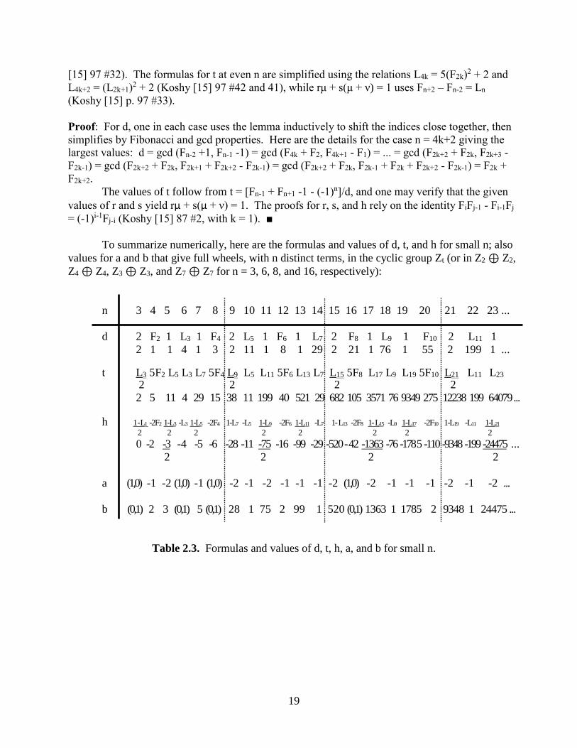
[15] 97 #32). The formulas for t at even n are simplified using the relations L4k = 5(F2k)2 + 2 and

L4k+2 = (L2k+1)2 + 2 (Koshy [15] 97 #42 and 41), while rμ + s(μ + ν) = 1 uses Fn+2 – Fn-2 = Ln

(Koshy [15] p. 97 #33).

Proof: For d, one in each case uses the lemma inductively to shift the indices close together, then

simplifies by Fibonacci and gcd properties. Here are the details for the case n = 4k+2 giving the

largest values: d = gcd (Fn-2 +1, Fn-1 -1) = gcd (F4k + F2, F4k+1 - F1) = ... = gcd (F2k+2 + F2k, F2k+3 -

F2k-1) = gcd (F2k+2 + F2k, F2k+1 + F2k+2 - F2k-1) = gcd (F2k+2 + F2k, F2k-1 + F2k + F2k+2 - F2k-1) = F2k +

F2k+2.

The values of t follow from t = [Fn-1 + Fn+1 -1 - (-1)n]/d, and one may verify that the given

values of r and s yield rμ + s(μ + ν) = 1. The proofs for r, s, and h rely on the identity FiFj-1 - Fi-1Fj

= (-1)i-1Fj-i (Koshy [15] 87 #2, with k = 1). ■

To summarize numerically, here are the formulas and values of d, t, and h for small n; also

values for a and b that give full wheels, with n distinct terms, in the cyclic group Zt (or in Z2 ⊕ Z2, Z4 ⊕ Z4, Z3 ⊕ Z3, and Z7 ⊕ Z7 for n = 3, 6, 8, and 16, respectively):

n 3 4 5 6 7 8 9 10 11 12 13 14 15 16 17 18 19 20 21 22 23 ...

d 2 F2 1 L3 1 F4 2 L5 1 F6 1 L7 2 F8 1 L9 1 F10 2 L11 1

2 1 1 4 1 3 2 11 1 8 1 29 2 21 1 76 1 55 2 199 1 ...

t L3 5F2 L5 L3 L7 5F4 L9 L5 L11 5F6 L13 L7 L15 5F8 L17 L9 L19 5F10 L21 L11 L23

2 2 2 2

2 5 11 4 29 15 38 11 199 40 521 29 682 105 3571 76 9349 275 12238 199 64079 ...

h 1-L1 -2F2 1-L3 -L3 1-L5 -2F4 1-L7 -L5 1-L9 -2F6 1-L11 -L7 1- L13 -2F8 1- L15 -L9 1-L17 -2F10 1-L19 -L11 1-L21

2 2 2 2 2 2 2 2

0 -2 -3 -4 -5 -6 -28 -11 -75 -16 -99 -29 -520 - 42 -1363 -76 -178 5 -110 -9348 -199 -24475 ...

2 2 2 2

a (1,0) -1 -2 (1,0) -1 (1,0) -2 -1 -2 -1 -1 -1 -2 (1,0) -2 -1 -1 -1 -2 -1 -2 ...

b (0,1) 2 3 (0,1) 5 (0,1) 28 1 75 2 99 1 520 (0,1) 1363 1 1785 2 9348 1 24475 ...

Table 2.3. Formulas and values of d, t, h, a, and b for small n.

20

3. Difference cographs

A difference cograph is a cograph in which the points are elements in either Z, with C(P,Q)

= |P-Q|, or in Zn, with C(P,Q) = min |p-q|, the minimum being taken over elements p in coset P and

q in coset Q. Figure 3.1 shows two examples:

1 2 1 2

0 3 5≡0 3

Over Z Over Z5

(single-copy edge C(0,3) not shown)

Fig. 3.1. Difference cographs on four points.

Difference cographs have some similarities to sum cographs, the points being again

basically just numbers, and the edges just differences rather than sums. But the absolute value

|P-Q| in difference cograph edges makes the latter class more complicated, and hence also more

numerous, because the simple configuration of Figure 3.2a forbidden in sum cographs can easily

occur, as both examples illustrate. (Configuration 3.2b continues to be forbidden,though.)

a) Allowed b) Forbidden

Fig. 3.2. Configurations allowed or forbidden in difference cographs.

Difference cographs are therefore better viewed not as algebraic, like sum cographs, but rather as

the simplest type of geometric (or “distance”) cographs: one-dimensional arrays of points and

distances measured along either a line or a circle.

Since any (finite) line segment can be wrapped into a semicircle, any (finite) difference

cograph can be considered part of a sufficiently large Zn. But the cographs embeddable in Z are a

specialized subclass, and will be distinguished from those (like the second example above) that

require torsion.

This section considers elementary properties and examples of difference cographs,

culminating in the complete listing of the 62 difference cographs on five points.

Lemma 3.1 (“Labeling”): A difference cograph may be relabeled to give any selected single point

any selected value in its group Z or Zn.

21

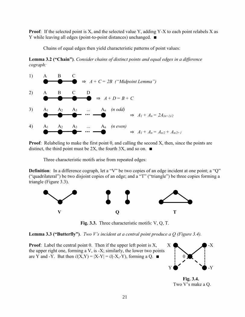
Proof: If the selected point is X, and the selected value Y, adding Y-X to each point relabels X as

Y while leaving all edges (point-to-point distances) unchanged. ∎

Chains of equal edges then yield characteristic patterns of point values:

Lemma 3.2 (“Chain”). Consider chains of distinct points and equal edges in a difference

cograph:

1) A B C

⇒ A + C = 2B (“Midpoint Lemma”)

2) A B C D

⇒ A + D = B + C

3) A1 A2 A3 ... An (n odd) ⇒ A1 + An = 2A(n+1)/2

4) A1 A2 A3 ... An (n even) ⇒ A1 + An = An/2 + An/2+1

Proof: Relabeling to make the first point 0, and calling the second X, then, since the points are

distinct, the third point must be 2X, the fourth 3X, and so on. ∎

Three characteristic motifs arise from repeated edges:

Definition: In a difference cograph, let a “V” be two copies of an edge incident at one point; a “Q”

(“quadrilateral”) be two disjoint copies of an edge; and a “T” (“triangle”) be three copies forming a

triangle (Figure 3.3).

V Q T

Fig. 3.3. Three characteristic motifs: V, Q, T.

Lemma 3.3 (“Butterfly”). Two V’s incident at a central point produce a Q (Figure 3.4).

Proof: Label the central point 0. Then if the upper left point is X, X -Xthe upper right one, forming a V, is -X; similarly, the lower two points

are Y and -Y. But then C(X,Y) = |X-Y| = C(-X,-Y), forming a Q. ∎ 0

Y -Y

Fig. 3.4. Two V’s make a Q.

22

Q’s are actually more complicated: there are five different types, all of which have at least

a second pair of repeated edges:

Lemma (“Q”): A Q in a difference cograph must be one of the five types in Figure 3.5:

a a+b x n/2 a 3a a 3a a 3a

0 b 0 x-n/2 0 2a 0 2a 0 2a in Z or Zn in Zn in Z or Zn in Z5a in Z4a

|a-b| ≠ |a+b|

Fig. 3.5. The five possibilities for a Q.

Proof: Each of the five labelings evidently yields a Q. If, conversely, 0, a, b, x are points with

C(0,a) = C(b,x) = and C(0,b) = C(a,x) = , then x = b ± a. The alternative x = b+a yields

the first type, while x = b-a gives C(0,x) = |a-b| = C(a,b), again the first type (or, for either case, the

second type if the diagonals are also equal). The third, fourth, and fifth cographs each contain a

chain of points that, by the chain lemma, may be labeled 0, a, 2a, 3a, hence satisfy

C(0,2a) = C(a,3a) = 2a = ≠ = a = C(0,a), the choice among the three types then

depending on the value of C(0,3a). ∎

As a corollary, observe that if A,B,C,D,E are five points in a difference E

cograph in which A,B,C,D form a Q, then if C(A,E) is any of the repeated edges

of the Q, the cograph must also contain a second Q (Figure 3.6). For the Q in A B

A,B,C,D must be one of the five types from the Q lemma, and if it is, say, the

first type, and C(A,E) = , then E,A,B,D will be a second Q. Hence in C D

cataloguing the five-point difference cographs, sorted by their number of Vs,

Qs, and Ts, requiring there to be just a single Q is a substantial restriction. Fig. 3.6. Two Q’s.

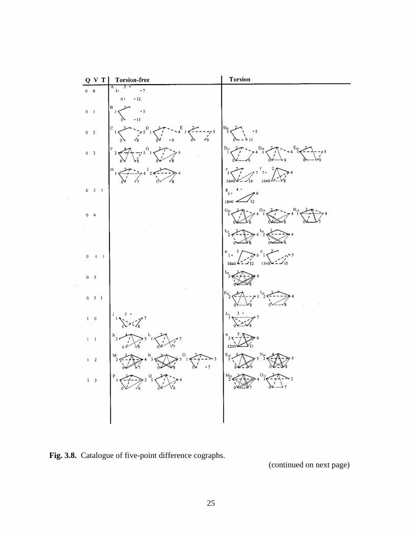
Catalogue Figures 3.7-3.8 below show the difference cographs (repeated edges only) on

two, three, four, or five points, sorted by whether the cographs require torsion or not, and by the

numbers of Qs, Vs, and Ts they contain. The legend gives details about the construction, point

labels, cograph names, and uniqueness, as well as a sketch of the proof that the five-point table is

complete.

Legend:

• Only multiple copy edges are shown.

• Point labels are low, but not rigorously checked to be least.

• Five-point cograph names:

The torsion-free cographs are sequentially named A-V.

23

Most of the torsion cographs can then be obtained by “reading” torsion-free structures in

some Zn (e.g. B20 is B read in Z20).

Nine torsion cographs cannot be so obtained: these are named arbitrarily c,f,g,n,o,u,f’,g’,

s’, and the appropriate cyclic group Zn is indicated explicitly by n ≡ 0 in each

diagram. Each of these nine can be obtained by reading an alternate equivalent

form of some torsion-free cograph in some Zn (e.g. C = 0 1 2 5 8 could also be

named--that is, is the same cograph as--Calt = 0 1 2 7 14, and Calt read in Z16 is c).

• The cograph sorting by Qs, Vs, and Ts, together with simple criteria like point “degrees” (= the

number of the multiple copy edges incident at each point), suffice to show that each cograph

in the table is unique.

A helpful technique here is “Doubling analysis” of edges, by which the

configuration implies that edge is twice edge . In the case of the five five-point

torsion cographs with Q = 0, V = 4, for example, one has:

G14: G15: H12: I13: I14:

showing at one glance that at least four of the five are distinct.

• The Q-V-T sorting then also gives the framework for a proof that the five-point cograph table is

complete.

Sketch of proof: At Q = 0, the butterfly lemma implies the Vs have distinct vertices, hence

V < 5. The most complicated case here is V = 3: If the five points are a,b,c,d,e, and (without loss

of generality) the three Vs have vertices a,b,c, then the V with vertex a--denote it Va--has (without

loss of generality) endpoints either b,c, or b,d, or d,e, whereas Vb and Vc each have six possible

choices for their pair of endpoints, and two or three possibilities for edges. Two general constraints

are:

1) If two Vs overlap (i.e., Vx has endpoints y,z, and Vy has endpoints x and w), they

consequently have the same edge, and wyxz consequently would form a Q (contradicting Q = 0)

unless w = z, forming a triangle; and

2) If Vx has endpoints y and z, and Vy has endpoints r and s, then the two Vs have different

edges (else point y would have the forbidden configuration of three identical edges incident at one

point).

One then checks that the individual cases (~84) all fall into the ten cases of the table.

At Q = 1, sorting by the five cases of the Q-lemma severely limits the possibilities,

especially when V = 5 or 6, and making V > 6 impossible.

At Q = 2, one finds that the two Q’s force there to be always at least one V, but that V > 5 is

impossible.

When Q = 3, one finds that the cograph must contain either a triangle and a pair with the

same edge, or else a 5-chain. These two constraints then are compatible only with the five

cographs in the table.

24

Fig. 3.7. Catalogue of two- three-, and four-point difference cographs.

25

Fig. 3.8. Catalogue of five-point difference cographs.

(continued on next page)

26

Fig. 3.8. Catalogue of five-point difference cographs.

(continued from previous page)

27

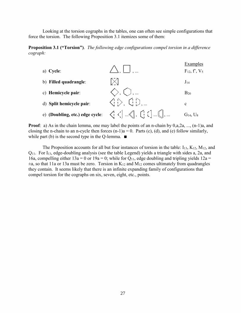
Looking at the torsion cographs in the tables, one can often see simple configurations that

force the torsion. The following Proposition 3.1 itemizes some of them:

Proposition 3.1 (“Torsion”). The following edge configurations compel torsion in a difference

cograph:

Examples

a) Cycle: , , ... F12, f’, V5

b) Filled quadrangle: J14

c) Hemicycle pair: , , ... B20

d) Split hemicycle pair: , , ... c

e) (Doubling, etc.) edge cycle: ... , ... , ... G14, U8

Proof: a) As in the chain lemma, one may label the points of an n-chain by 0,a,2a, ..., (n-1)a, and

closing the n-chain to an n-cycle then forces (n-1)a = 0. Parts (c), (d), and (e) follow similarly,

while part (b) is the second type in the Q-lemma. ∎

The Proposition accounts for all but four instances of torsion in the table: I13, K12, M12, and

Q11. For I13, edge-doubling analysis (see the table Legend) yields a triangle with sides a, 2a, and

16a, compelling either 13a = 0 or 19a = 0; while for Q11, edge doubling and tripling yields 12a =

±a, so that 11a or 13a must be zero. Torsion in K12 and M12 comes ultimately from quadrangles

they contain. It seems likely that there is an infinite expanding family of configurations that

compel torsion for the cographs on six, seven, eight, etc., points.

28

Remark: 2-Dimensional Four-Point Cographs

As proved in Theorem 1.1, every finite cograph can be realized as a geometric cograph of

sufficiently high dimension. That I have not explored geometric cographs beyond difference

cographs, the one-dimensional simplest case, is undoubtedly due to my own limitations (as by

nature an algebraist, not a geometer), not the subject’s. As a glimpse ahead, it is straightforward to

show that only one of the 25 possible four-point cographs, Figure 3.9, cannot be realized

geometrically in two dimensions. The 24 realizations are mostly quite immediate, the most

challenging being Figure 3.10.

Fig. 3.9. Cannot be realized Fig. 3.10. Challenging

in two dimensions. to realize in two dimensions.

A realization of Figure 3.10--the only possible one, up to rigid motions, scaling, and switching the

two sides x and y--is Figure 3.11:

y

P S

Q R

T x U

Fig. 3.11. Geometric realization of the cograph of Fig. 3.10.

where the angles QPR, RPS, PSQ, QSR, SQR, and PRQ are π/5; PQT, PQS, POQ, SOR, SRP, and

SRU are 2π/5; POS and QOR are 3π/5; and TPQ and RSU are π/10; and consequently y =

(1+ 2 sin π/10) x ≈ 1.618 x. Drawing the bisector of PRS, to cut PS at a point V, in fact yields an

isosceles triangle VRS similar to RPS, proving that PRS is a so-called “golden triangle,” with ratio

of sides y/x equal to the “golden ratio” φ ≈ 1.618 that is a root (1+ √5)/2 of the equation φ2 =

φ + 1.

O

29

4.1. Intersection cographs

An intersection cograph is a cograph in which the points and edges are sets, and each edge

is the intersection of its two endpoints. Catalogue Figure 4.1.6 below gives the fifteen four-point

intersection cographs (showing only the multiple-copy edges). That these cographs are all that are

possible on four points will follow from a simple intersection cograph property:

Proposition 4.1.1 (Quadrilateral rule). Every quadrilateral abcd in an a

intersection cograph satisfies a ∩ c = b ∩ d. P Q

d b

Proof: Call the points of the quadrilateral P, Q, R, and S (Fig. 4.1.1). S R

Then a ∩ c = P ∩ Q ∩ R ∩ S = b ∩ d. ∎ c

Fig. 4.1.1.

Corollary: The configurations of Figure 4.1.2 in an intersection Quadrilateral abcd.

cograph each imply a ⊃ b. a a

Proof: Letting d = b in Proposition 4.1.1, b b

a ⊃ a ∩ c = b ∩ d = b ∩ b = b; the second

part is similar. ∎ Fig. 4.1.2. Configurations

that imply a ⊃ b.

a b c n b c d . . . a

Fig. 4.1.3. A forbidden “inclusion cycle.”

Any “inclusion cycle” of distinct edges as in Figure 4.1.3 is therefore forbidden in an intersection

cograph, since it would entail a ⊃ b ⊃ c ⊃ d ⊃ ... n ⊃ a, forcing a = b = c = d = ... = n, which

contradicts the assumption that the edges are distinct. The two

simplest such forbidden configurations have cycle lengths two and three (Figure 4.1.4). Checking the Figure 1.2 listing of all 25 four-point cographs, one sees that every one omitted from the

intersection cographs contains one of these forbidden configurations. Fig. 4.1.4 Two simple forbidden configurations. Inclusion cycles are not the only type of obstruction, though:

a a a b c a b c

a ⊃ b a ⊃ c a ∩ b = a ∩ c

Fig. 4.1.5. Another type of obstruction.

The simple 12-point configuration of Figure 4.1.5 is forbidden in an intersection cograph too, since

it yields the contradiction b = a ∩ b = a ∩ c = c. And the forbidden configuration can actually be

packed into just six points, as in Figure 4.1.7.

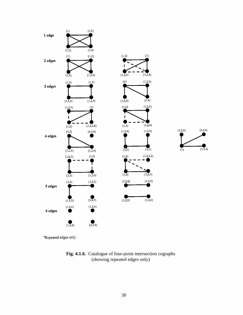
30

Fig. 4.1.6. Catalogue of four-point intersection cographs

(showing repeated edges only)

31

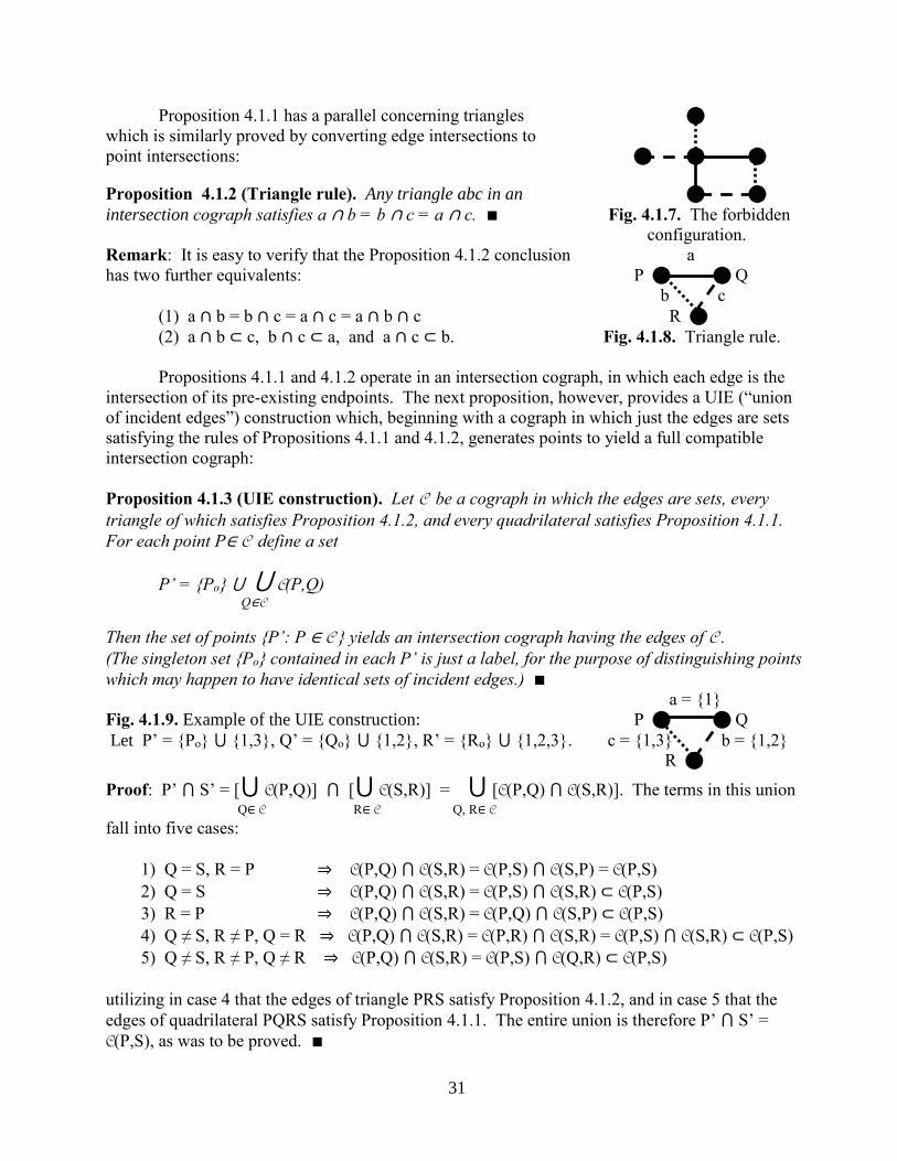
Proposition 4.1.1 has a parallel concerning triangles

which is similarly proved by converting edge intersections to point intersections: Proposition 4.1.2 (Triangle rule). Any triangle abc in an

intersection cograph satisfies a ∩ b = b ∩ c = a ∩ c. ∎ Fig. 4.1.7. The forbidden

configuration.

Remark: It is easy to verify that the Proposition 4.1.2 conclusion a

has two further equivalents: P Q

b c

(1) a ∩ b = b ∩ c = a ∩ c = a ∩ b ∩ c R

(2) a ∩ b ⊂ c, b ∩ c ⊂ a, and a ∩ c ⊂ b. Fig. 4.1.8. Triangle rule.

Propositions 4.1.1 and 4.1.2 operate in an intersection cograph, in which each edge is the

intersection of its pre-existing endpoints. The next proposition, however, provides a UIE (“union

of incident edges”) construction which, beginning with a cograph in which just the edges are sets

satisfying the rules of Propositions 4.1.1 and 4.1.2, generates points to yield a full compatible

intersection cograph:

Proposition 4.1.3 (UIE construction). Let C be a cograph in which the edges are sets, every

triangle of which satisfies Proposition 4.1.2, and every quadrilateral satisfies Proposition 4.1.1.

For each point P∈ C define a set

P’ = {Po} ⋃ ⋃ C(P,Q) Q∈C

Then the set of points {P’: P ∈ C } yields an intersection cograph having the edges of C .

(The singleton set {Po} contained in each P’ is just a label, for the purpose of distinguishing points

which may happen to have identical sets of incident edges.) ∎

a = {1}

Fig. 4.1.9. Example of the UIE construction: P Q

Let P’ = {Po} ⋃ {1,3}, Q’ = {Qo} ⋃ {1,2}, R’ = {Ro} ⋃ {1,2,3}. c = {1,3} b = {1,2}

R

Proof: P’ ⋂ S’ = [⋃ C(P,Q)] ⋂ [⋃ C(S,R)] = ⋃ [C(P,Q) ⋂ C(S,R)]. The terms in this union Q∈ C R∈ C Q, R∈ C

fall into five cases:

1) Q = S, R = P ⇒ C(P,Q) ⋂ C(S,R) = C(P,S) ⋂ C(S,P) = C(P,S)

2) Q = S ⇒ C(P,Q) ⋂ C(S,R) = C(P,S) ⋂ C(S,R) ⊂ C(P,S)

3) R = P ⇒ C(P,Q) ⋂ C(S,R) = C(P,Q) ⋂ C(S,P) ⊂ C(P,S)

4) Q ≠ S, R ≠ P, Q = R ⇒ C(P,Q) ⋂ C(S,R) = C(P,R) ⋂ C(S,R) = C(P,S) ⋂ C(S,R) ⊂ C(P,S)

5) Q ≠ S, R ≠ P, Q ≠ R ⇒ C(P,Q) ⋂ C(S,R) = C(P,S) ⋂ C(Q,R) ⊂ C(P,S)

utilizing in case 4 that the edges of triangle PRS satisfy Proposition 4.1.2, and in case 5 that the

edges of quadrilateral PQRS satisfy Proposition 4.1.1. The entire union is therefore P’ ⋂ S’ =

C(P,S), as was to be proved. ∎

32

Remark 1: The UIE-constructed cograph is not unique, but it is minimal: If {P”} also has

intersection cograph C, then for each P, P” P’ - {Po}, and the elements of P” - P’ are not

contained in any other Q” - Q’, else they would appear in the intersection P” ⋂ Q”.

Remark 2: An example illustrates the issue of representing an abstract cograph a

as an intersection cograph. Consider the abstract cograph PQRS of Fig. 4.1.10. P Q

Its edges form triangles aaa (from PQS), abb (from PQR), and abc (from SPR and b

SQR), and quadrilaterals abca (from PQRS), bbaa (from PRQS), and bcaa (from S R

PRSQ). While triangle aaa yields no information, abb implies a ⋂ b = b ⋂ b = b, c

forcing b ⊂ a (see the Corollary to Proposition 4.1.1), and abc then yields (see Fig. 4.1.10.

Proposition 4.1.2) that a ⋂ c = a ⋂ b = b. Since the three qadrilaterals turn out to Example of

contribute no further information, the general solution is to select a and c arbitrarily representation

and let b = a ⋂ c. A satisfactory set representation is thus a = {1,2}, c = {1,3},

b = {1}; and UIE-constructed points P = {1,2}, Q = {1,2,4} (the element 4 added to

distinguish it from P), R = {1,3}, and S = {1,2,3}.

33

4.2. Intersection cographs and aesthetics

Mathematics is such a beautiful subject it is not surprising that many mathematicians have

been strongly moved by beauty, and a number of them have devised mathematical formulations of

aesthetics. For instance, H. Weyl’s book Symmetry traces the role of group theoretical symmetry in

the visual arts [19], while Birkhoff offers a definition of beauty through a concept of "aesthetic

measure" [4]. To a degree, of course, "beauty is in the eye of the beholder"; that is, the beauty

must arise not solely from the beautiful object itself, but rather in the interaction of that object with

the percipient, in the act of perception. This section will suggest how intersection cographs might

offer a mathematical model for that interaction.

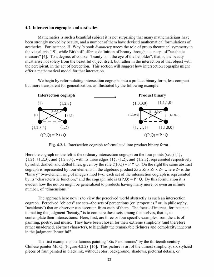
We begin by reformulating intersection cographs into a product binary form, less compact

but more transparent for generalization, as illustrated by the following example:

Intersection cograph Product binary

C(P,Q) = P ∩ Q C(P,Q) = P . Q

Fig. 4.2.1. Intersection cograph reformulated into product binary form.

Here the cograph on the left is the ordinary intersection cograph on the four points (sets) {1},

{1,2}, {1,2,3}, and {1,2,3,4}, with its three edges {1}, {1,2}, and {1,2,3}, represented respectively

by solid, dashed, and dotted lines, given by the rule C(P,Q) = P ∩ Q. On the right the same abstract

cograph is represented by four elements in the algebraic product Z2 x Z2 x Z2 x Z2, where Z2 is the

“binary” two-element ring of integers mod two; each set of the intersection cograph is represented

by its “characteristic function,” and the cograph rule is C(P,Q) = P . Q. By this formulation it is

evident how the notion might be generalized to products having many more, or even an infinite

number, of “dimensions.” The approach here now is to view the perceived world abstractly as such an intersection

cograph. Perceived "objects" are sets--the sets of perceptions (or "properties," or, in philosophy,

“accidents”) that an observer can ascertain from each of them. The focus of interest, for instance,

in making the judgment "beauty," is to compare these sets among themselves, that is, to

contemplate their intersections. Here, first, are three or four specific examples from the arts of

painting, poetry, and music. They have been chosen for their extreme simplicity (and therefore

rather unadorned, abstract character), to highlight the remarkable richness and complexity inherent

in the judgment "beautiful".

The first example is the famous painting "Six Persimmons" by the thirteenth century

Chinese painter Mu Qi (Figure 4.2.2) [16]. This picture is art of the utmost simplicity: six stylized

pieces of fruit painted in black ink, without color, background, shadows, pictorial details, or

{1}

{1,2,3}

{1,2,3,4}

{1,2}

{1}

{1,2}

{1,2,3}

{1,1,1,1}

{1,1,0,0}

{1,1,1,0}

{1,0,0,0}

{1,0,0,0}

{1,1,0,0}

{1,1,1,0}

34

Fig. 4.2.2. Mu Qi: “Six Persimmons,” 13th c. Chinese.

35

dramatic perspective. It can, nevertheless, arouse a powerful emotional response in a sensitive

viewer: "passion ... congealed into a stupendous calm," is the reaction of one critic [18].

Intersection cographs can describe the process of perception as the appreciating eye plays over this

picture:

Persimmon 1 2 3 4 5 6

Aspect

a Frontality 0 0 1 0 0 0

b Frontality’ 0 1 1 0 0 0

c Frontality” 0 1 2 1 1 0

d Color 0 1 1 3 2 0

e Size 1 1 0 2 1 1

f Shape 0 1 1 2 2 1

g Stem 2 2 1 3 1 2

Fig. 4.2.3. Aspects of Mu Qi’s “Six Persimmons.”

The first line of the figure shows the result of the first glance (Aspect a): Of the six persimmons in

the picture, numbers 1, 2, and 4, 5, 6 share the characteristic of being in one row in back, while

number 3 is further to the front. Aspect b gives the second closer glance: fruit 2 is slightly ahead

of the rest of the back row, and thus is united in similarity with number 3. Aspect c gives the most

detailed look: the persimmons at both ends are subtly overlapped, hence behind the adjacent fruits.

As one studies the painting, first one fruit and then another catches the eye, gaining prominence not

only from position, but also by size, shape, or shading. Aspect d shows the cograph for color: the

two fruits at the ends share the palest color, the fourth is darkest, the others are intermediate.

Aspect e shows size; aspect f shape--oval, round, or squarish. Aspect g compares the lengths of

the stems of the fruits. All of us become amateur artists when we make photos, and triumph when

we center our friends in a snapshot. In his picture Mu-Qi has "balanced" all seven different aspects

of position, shape, color, ... (and there are more) described in the cographs. The composition

would be destroyed by omitting any one of the six fruits, and ruined by so much as shifting any

position, size, shape, or color. It is this perfect equipoise of strong figural forces that produces the

feeling of calm and passion noted by the critic; it is this exquisite balance that makes the painting a

great work of art.

A similar balance characterizes the beauty of a poem. The example here is a verse from a

lyric by Emily Dickinson (the first poem she valued highly enough to send to a critic [7])

describing the noble repose of the redeemed dead awaiting their resurrection on Judgment Day:

Safe in their Alabaster Chambers--

Untouched by Morning--

And untouched by Noon--

Sleep the meek members of the Resurrection,

Rafter of Satin--and Roof of Stone--

The first impression one receives in reading this poem is perhaps the rhythm (Figure 4.2.4, Aspect

a). The idiomatically mixed dactylic (‾ ˘ ˘) and trochaic (‾ ˘) pulse carries the words along to make

them "verse" rather "prose", while placing special emphasis on emotionally important words like

36






Aspect a: Rhythm Aspect b: Vowel assonances

Aspect c: Consonant alliteration Aspect d: Sense

Fig. 4.2.4. Aspects of the Dickinson poem “Safe in their Alabaster Chambers.”

"safe," "untouched," and "sleep." The rhythm alone creates the powerful effect in the last line,

where the drumbeat of the dactylic "Rafter of Satin" (‾ ˘ ˘ ‾ ˘) slows to the iambics "and Roof of

Stone" (˘ ‾ ˘ ‾) to produce a feeling of unshakable solidity and firmness that will outlast the eons.

Reinforcing the poem’s initial rhythmic pattern then is the music of the language itself.

Aspect b summarizes the vowel rhymes and assonances; these, for example, link "Safe" to

"Chambers" in the first line, "Sleep" to "meek" as an internal rhyme in the fourth, and "Alabaster"

in the first to "Rafter" and "Satin" in the last. The consonantal alliterations (Aspect c) provide even

more numerous linkages. For example, the "s" sound in the first word "Safe" is echoed in

"Alabaster," "Chambers," "Sleep," "members," "Resurrection," "Satin," and the last word "Stone."

The "m," "r," and "t" sounds recur similarly. The alliterations also contribute notably to the effect

of the last line, where the "r," "f," "s," "t," and "n" of "Rafter of Satin" are echoed exactly by those

in "Roof of Stone."

Poetry, finally, requires a harmony of sense mutually reinforcing that of sound. Aspect d

indicates some of the sense patterns in this lyric: The central thought is how the physical

environment ("Chambers," "Rafter," and "Roof"), charged with emotional connotations of

protection and permanence ("Alabaster", "Satin," "Stone"), shields its inhabitants from time

("Morning," "Noon," and "Resurrection"). The great majority of words in the lyric express this

protection: "Safe," "Alabaster," "Chambers," "Untouched," "Untouched," "Sleep," "Meek,"

"Rafter," and "Roof." As with the "Six Persimmons" painting, this lyric is created from only a few

ingredients. The exquisite rightness and economy of its crafting, each word linked to the others in

a balance of rhythm, sound, and sense, make it, too, a great work of art.

Though this example deals with the minutest elements of sound and meaning, intersection

cographs also easily represent much larger literary structures. For example, the cograph of Figure

4.2.5, with solid, dashed, or invisible white line segments, shows the main characters and

relationships in Shakespeare’s play King Lear:






‾ ˘ ˘ ‾ ˘ ‾ ˘ ‾ ˘ ‾ ˘ ˘ ‾ ˘ ˘ ‾ ˘ ˘ ‾ ‾ ˘ ‾ ‾ ˘ ˘ ˘ ˘ ˘ ‾ ˘ ‾ ˘ ˘ ‾ ˘ ˘ ‾ ˘ ‾











37

Lear Gloucester

● ●

● ● ● ● ●

Goneril Regan Cordelia Edgar Edmund

Fig. 4.2.5. Cograph of characters in Shakespeare’s King Lear.

The central issue in this play, announced already in its third line “Is not this your son, my lord?”, is

the nature of the relationship between parent and child. The cograph schematizes, graphically and

instantaneously, the two forms occurring here: the false one, between Lear and Goneril, Lear and

Regan, and Gloucester and Edmund, and the true one, between Lear and Cordelia, and Gloucester

and Edgar.

The final example is a musical one. It is difficult to find a profound piece of music on as

miniature a scale as the Mu Qi painting or the Dickinson lyric, and we will content ourselves with a

fragment, the first eight measures of the familiar beginner's minuet in G from the notebook of Anna

Magdalena Bach (Fig. 4.2.6) [2]. Music, like poetry but unlike painting, is organized along a

strictly linear pattern extended in time. Its first impression is therefore also the underlying

rhythmical pattern. The rhythm is stricter for music than poetry, and the first rhythm cograph (not

shown) simply records its steady 1-2-3 pattern of beats. This strict foundation, however, then

permits the elaboration of more complex hierarchical structures: Fig. 4.2.7a highlights the repeated

figure of four eighth notes leading up to a quarter note. Coincident with the rhythmic patterns are

melodic and harmonic ones. Musical analysis (pioneered most formally by Schenker [8]) reveals

these latter patterns most clearly by "rhythmic reduction" which omits ornamental filigree notes.

The underlying pattern then stands out clearly: here, two simple scale passages, ascending, then

descending to the tonic note G (Fig. 4.2.7b - circled notes). Other dimensions of musical

expression include the shading of dynamics, ranging from soft to loud; progression of the

underlying harmonies; small but important adjustments in tempo, such as ritards or accelerandos

near musical climaxes; and, in ensemble music, use of the palette of colors of the different

instruments. As with the other arts, an aesthetically satisfying musical composition or performance

will be one in which the multiple dimensions of structure summarized schematically by the

cographs are integrated into a convincing whole.

Fig. 4.2.6. Beginning of the Minuet in G, from the notebook of Anna Magdalena Bach.

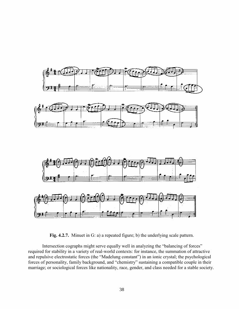
38

Fig. 4.2.7. Minuet in G: a) a repeated figure; b) the underlying scale pattern.

Intersection cographs might serve equally well in analyzing the “balancing of forces”

required for stability in a variety of real-world contexts: for instance, the summation of attractive

and repulsive electrostatic forces (the “Madelung constant”) in an ionic crystal; the psychological

forces of personality, family background, and “chemistry” sustaining a compatible couple in their

marriage; or sociological forces like nationality, race, gender, and class needed for a stable society.

39

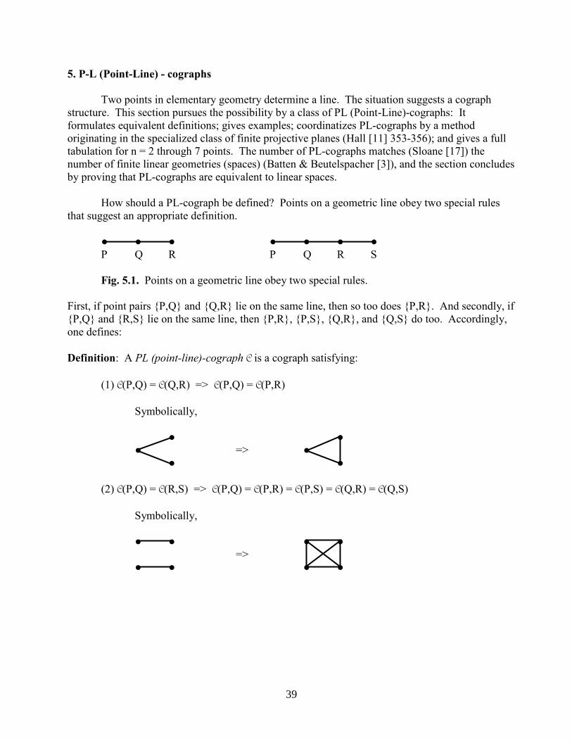
5. P-L (Point-Line) - cographs

Two points in elementary geometry determine a line. The situation suggests a cograph

structure. This section pursues the possibility by a class of PL (Point-Line)-cographs: It

formulates equivalent definitions; gives examples; coordinatizes PL-cographs by a method

originating in the specialized class of finite projective planes (Hall [11] 353-356); and gives a full

tabulation for n = 2 through 7 points. The number of PL-cographs matches (Sloane [17]) the

number of finite linear geometries (spaces) (Batten & Beutelspacher [3]), and the section concludes

by proving that PL-cographs are equivalent to linear spaces.

How should a PL-cograph be defined? Points on a geometric line obey two special rules

that suggest an appropriate definition.

● ● ● ● ● ● ●

P Q R P Q R S

Fig. 5.1. Points on a geometric line obey two special rules.

First, if point pairs {P,Q} and {Q,R} lie on the same line, then so too does {P,R}. And secondly, if

{P,Q} and {R,S} lie on the same line, then {P,R}, {P,S}, {Q,R}, and {Q,S} do too. Accordingly,

one defines:

Definition: A PL (point-line)-cograph C is a cograph satisfying:

(1) C(P,Q) = C(Q,R) => C(P,Q) = C(P,R)

Symbolically,

● ●

● => ●

● ●

(2) C(P,Q) = C(R,S) => C(P,Q) = C(P,R) = C(P,S) = C(Q,R) = C(Q,S)

Symbolically,

● ● ● ●

=>

● ● ● ●

40

(A) ● ● (All unmarked edges are single-copy)

●

● ●

●

(B) ●

● ●

● ●

Fig. 5.2. Two simple counterexamples (not PL-cographs) show that the defning conditions for PL-

cographs are independent: (A) satisfies condition 1 but not 2; (B) satisfies condition 2 but not 1.

2

A ●

1 ● ● 3 (The three unmarked edges C(1,4) = E, C(2,5) = F, and C C(3,6) = G are single-copy.) B D 6 ● ●4

●

5

Fig. 5.3. Example: A six-point seven-edge PL-cograph.

Visualizing the figure as an octahedron makes it evident that the four edges A, B, C, and D are

equivalent.

Figure 5.5 further below shows all the PL-cographs on n < 7 points.

In studying PL-cographs it is useful to consider the graphs--term them blocks--formed by

single edges and their endpoints. The definition of a PL-cograph is that every 3- or 4-point block is

a complete graph. Here are some equivalent characterizations by these terms:

Proposition 5.1. The following four characterizations of a PL-cograph are equivalent:

1) ● ● ● ● ● ●

● => ● and =>

● ● ● ● ● ●

2) Every 3- or 4-point block is a complete graph.

3) Every block is a complete graph.

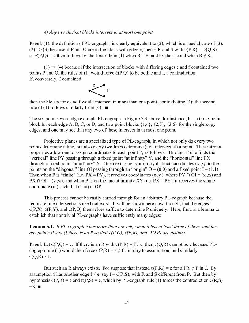
41

4) Any two distinct blocks intersect in at most one point.

Proof: (1), the definition of PL-cographs, is clearly equivalent to (2), which is a special case of (3).

(2) => (3) because if P and Q are in the block with edge e, then R and S with C(P,R) = C(Q,S) =

e. C(P,Q) = e then follows by the first rule in (1) when R = S, and by the second when R ≠ S.

(1) => (4) because if the intersection of blocks with differing edges e and f contained two

points P and Q, the rules of (1) would force C(P,Q) to be both e and f, a contradiction.

If, conversely, C contained

e ●

● f

●

then the blocks for e and f would intersect in more than one point, contradicting (4); the second

rule of (1) follows similarly from (4). ■

The six-point seven-edge example PL-cograph in Figure 5.3 above, for instance, has a three-point

block for each edge A, B, C, or D, and two-point blocks {1,4}, {2,5}, {3,6} for the single-copy

edges; and one may see that any two of these intersect in at most one point.

Projective planes are a specialized type of PL-cograph, in which not only do every two

points determine a line, but also every two lines determine (i.e., intersect at) a point. These strong

properties allow one to assign coordinates to each point P, as follows. Through P one finds the

“vertical” line PY passing through a fixed point “at infinity” Y, and the “horizontal” line PX

through a fixed point “at infinity” X. One next assigns arbitrary distinct coordinates (xi,xi) to the

points on the “diagonal” line OI passing through an “origin” O = (0,0) and a fixed point I = (1,1).

Then when P is “finite” (i.e. PX ≠ PY), it receives coordinates (xi,yi), where PY ∩ OI = (xi,xi) and

PX ∩ OI = (yi,yi), and when P is on the line at infinity XY (i.e. PX = PY), it receives the single

coordinate (m) such that (1,m) OP.

This process cannot be easily carried through for an arbitrary PL-cograph because the

requisite line intersections need not exist. It will be shown here now, though, that the edges

C(P,X), C(P,Y), and C(P,O) themselves suffice to determine P uniquely. Here, first, is a lemma to

establish that nontrivial PL-cographs have sufficiently many edges:

Lemma 5.1. If PL-cograph C has more than one edge then it has at least three of them, and for

any points P and Q there is an R so that C(P,Q), C(P,R), and C(Q,R) are distinct.

Proof: Let C(P,Q) = e. If there is an R with C(P,R) = f ≠ e, then C(Q,R) cannot be e because PL-

cograph rule (1) would then force C(P,R) = e ≠ f contrary to assumption; and similarly,

C(Q,R) ≠ f.

But such an R always exists. For suppose that instead C(P,Ri) = e for all Ri ≠ P in C. By

assumption C has another edge f ≠ e, say f = C(R,S), with R and S different from P. But then by

hypothesis C(P,R) = e and C(P,S) = e, which by PL-cograph rule (1) forces the contradiction C(R,S)

= e. ■

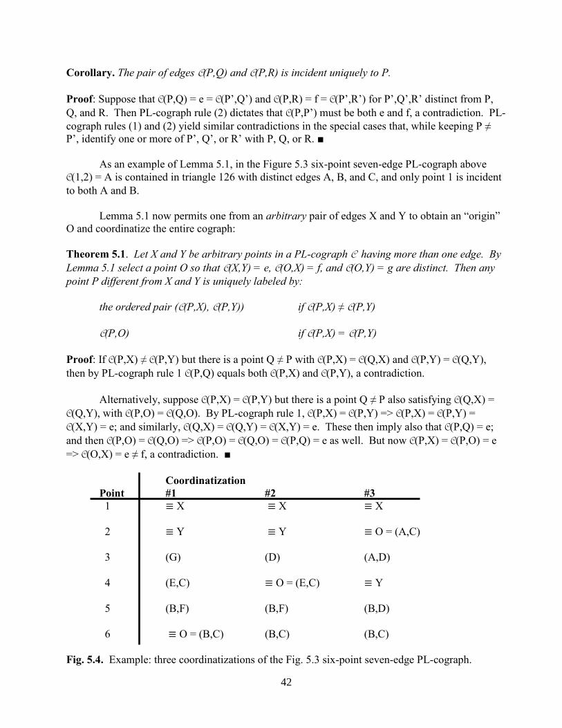
42

Corollary. The pair of edges C(P,Q) and C(P,R) is incident uniquely to P.

Proof: Suppose that C(P,Q) = e = C(P’,Q’) and C(P,R) = f = C(P’,R’) for P’,Q’,R’ distinct from P,

Q, and R. Then PL-cograph rule (2) dictates that C(P,P’) must be both e and f, a contradiction. PL-

cograph rules (1) and (2) yield similar contradictions in the special cases that, while keeping P ≠

P’, identify one or more of P’, Q’, or R’ with P, Q, or R. ■

As an example of Lemma 5.1, in the Figure 5.3 six-point seven-edge PL-cograph above

C(1,2) = A is contained in triangle 126 with distinct edges A, B, and C, and only point 1 is incident

to both A and B.

Lemma 5.1 now permits one from an arbitrary pair of edges X and Y to obtain an “origin”

O and coordinatize the entire cograph:

Theorem 5.1. Let X and Y be arbitrary points in a PL-cograph C having more than one edge. By

Lemma 5.1 select a point O so that C(X,Y) = e, C(O,X) = f, and C(O,Y) = g are distinct. Then any

point P different from X and Y is uniquely labeled by:

the ordered pair (C(P,X), C(P,Y)) if C(P,X) ≠ C(P,Y)

C(P,O) if C(P,X) = C(P,Y)

Proof: If C(P,X) ≠ C(P,Y) but there is a point Q ≠ P with C(P,X) = C(Q,X) and C(P,Y) = C(Q,Y),

then by PL-cograph rule 1 C(P,Q) equals both C(P,X) and C(P,Y), a contradiction.

Alternatively, suppose C(P,X) = C(P,Y) but there is a point Q ≠ P also satisfying C(Q,X) =

C(Q,Y), with C(P,O) = C(Q,O). By PL-cograph rule 1, C(P,X) = C(P,Y) => C(P,X) = C(P,Y) =

C(X,Y) = e; and similarly, C(Q,X) = C(Q,Y) = C(X,Y) = e. These then imply also that C(P,Q) = e;

and then C(P,O) = C(Q,O) => C(P,O) = C(Q,O) = C(P,Q) = e as well. But now C(P,X) = C(P,O) = e

=> C(O,X) = e ≠ f, a contradiction. ■

Coordinatization

Point #1 #2 #3

1 ≡ X ≡ X ≡ X

2 ≡ Y ≡ Y ≡ O = (A,C)

3 (G) (D) (A,D)

4 (E,C) ≡ O = (E,C) ≡ Y

5 (B,F) (B,F) (B,D)

6 ≡ O = (B,C) (B,C) (B,C)

Fig. 5.4. Example: three coordinatizations of the Fig. 5.3 six-point seven-edge PL-cograph.

43

In #1 C(X,Y), C(X,O), and C(Y,O) are all multiple-copy; in #2 C(X,O) is single-copy; in #3 C(X,Y)

is single-copy. Note that #1 and 2 have an “infinite” (single-coordinate) point, but #3 does not.

Theorem 5.1 and the example thus show that coordinatizing a PL-cograph by edges is a

natural and straightforward process. Coordinatization via point coordinates, in contrast, is complex

and problematic, requiring the PL-cograph or its equivalent linear geometry to be embedded in a

(possibly infinite) projective plane via some of the deepest and most difficult theorems in the field

(Batten & Beutelspacher [3]). Edge-coordinatization is even sometimes possible in cases more

general than PL-cographs: In Counterexample 1 (but not 2) above, for instance, the sets of incident

edges determine each point uniquely.

Figure 5.5 below shows all the PL-cographs on n < 7 points. Some PL-cographs fall into

families--for instance, n-point cographs Sn have all edges single-copy, while n-point cographs Kn

have just one edge (thus forming complete graphs). Small PL-cographs can combine into larger

ones, and the table also illustrates naming cographs by decomposition under two natural operations

+ and ∨:

Definitions: Let C and D be PL-cographs, where the n points and e edges of C are distinct from the

m points and f edges of D. Then define C + D to have point set the union of the point sets of C and

D, with (C + D)(P,Q) = C(P,Q) if P and Q are both in C, D(P,Q) if P and Q are both in D, and a new

single-copy edge e{P,Q} if P ∈ C and Q ∈ D or if P ∈ D and Q ∈ C. C + D thus has n + m points and e

+ f + nm edges.

Similarly, if all the points of C and of D are equivalent (i.e. if C and D have either just one

edge, or all single-copy edges), define C ∨ D to have for its n + m - 1 points the points of C and of D

joined at one point, with (C ∨ D)(P,Q) = C(P,Q) if P and Q are both in C ~ D, D(P,Q) if P and Q are

both in D ~ C, and a new single-copy edge e{P,Q} otherwise. C ∨ D thus has n + m - 1 points and

e + f + (n-1)(m-1) edges.

Examples: As shown in Figure 5.5, K3 + K3 is a 6-point 11-edge “prism,” and K3 ∨ K3 is a 5-point

6-edge “butterfly.”

The number of PL-cographs on n points is:

n 2 3 4 5 6 7 8 9

PL-cographs 1 2 3 5 10 24 69 384

n 10 11 12

PL-cographs 5250 232929 28872973

Here the values for n = 2 through 7 are from Figure 5.5, and for 8 through 12 are from sequence

A001200 of the Sloane On-line Encyclopedia of Integer Sequences, “number of linear geometries

on n points,” with which the n = 2 through 7 values (non-uniquely) match. The table will thus be

justified by Theorem 5.2 below identifying PL-cographs with linear spaces (geometries).

44

Fig. 5.5. Catalogue of PL-cographs.

(continued next page)

45

Fig. 5.5. Catalogue of PL-cographs.


46

A linear space S = (p,L) is defined (Batten & Beutelspacher [3]) as a set of “points” p and a

set of “lines” L (a line being a set of points) so that:

(1) any two distinct points belong to exactly one line

(2) every line has at least two points.

Theorem 5.2. Linear spaces are equivalent to PL-cographs.

Proof: From a linear space S = (p, L) one may form a cograph C with points the points p of S, edges

the lines L of S, and C(P,Q) the unique line of S passing through P and Q. The properties making

C a PL-cograph then follow because the lines of S are sets.

Conversely, a PL-cograph C yields a linear space S = (p, L) where p is the points of C, and

the line through P and Q is the set of all endpoints of the edge C(P,Q). The PL-cograph rules

guarantee that this is well-defined, and that S is then a linear space.

These two transformations, of linear space to PL-cograph and then back, are easily checked

to be inverses, so the two structures are in 1-1 correspondence. ■

PL-cograph blocks correspond under this theorem to linear space lines. Thus, for example,

Proposition 5.1(4): two blocks intersect in at most one point, becomes: two lines intersect in at

most one point.

For completeness, Figure 5.6 below presents the linear spaces on n < 7 points

corresponding to, and in the same order as, the PL-cographs of Figure 5.5. The point-and-line

notation of Figure 5.6 is more efficient for the specialized class of linear spaces than the more

general modified cograph notation of Figure 5.5, because it does not “fill in” the blocks. For

example, linear spaces in the family Kn are simply those with all their points on one line.

The situation suggests a new classification of the linear spaces, sorting them by the number

of nontrivial lines (blocks) containing three or more points. Each family is then infinite--e.g., there

are one-line spaces Kn for n = 3,4,..., 2-line spaces with n = 5,6,... points, etc. But in a 2-line space

the two lines may have either 0 or 1 intersection, in 3-line spaces the lines may be either all

parallel, have one intersection, two intersections, or form a triangle, and so on. In other words, one

may classify the linear spaces as arising through expansion by adding points (but not nontrivial

lines) from “minimal” spaces (having each point on a nontrivial line, and not expanded from any

smaller such space). The minimal spaces in Figure 5.6 are marked by ❋. Using the table of linear

spaces compiled by Jean Doyen (Batten & Beutelspacher [3]), slightly extended, then yields the

following enumeration of minimal linear spaces, in terms of their points or nontrivial lines:

n 1 2 3 4 5 6 7 8 9

minimal linear spaces:

on n points 0 0 1 0 1 3 8 23 208

with n non-trivial lines 1 2 5 16 >70

The Sloane Encyclopedia does not appear to contain geometry sequences matching either of these,

suggesting the minimality approach may be new.

47

Fig. 5.6. Catalogue of linear spaces.

(continued next page)

48

Fig. 5.6. Catalogue of linear spaces.


49

6. Group cographs: Ladders, chains, and chain groups

An (additive) abelian group naturally becomes a cograph, as illustrated in Figure 1.4 above,

when one defines the edge between each pair of points P and Q to be their sum P+Q. In a general

(multiplicative) group, though, there are two possible products PQ and QP, with no evident way to

prefer one over the other. To make the group a cograph, one therefore takes the set of both:

Definition: The group cograph C over a group G has as its points the elements of the group, with

C(P,Q) = {PQ,QP}.

This section discusses the ladders and chains that characteristically arise from multiple-copy edges

in a group cograph, and then solves the interesting group-theoretic problem of characterizing the

chain group generated in a finite group from terms that produce a chain.

The first theorem shows how any repeated edge in a group cograph yields whole ladders of

repeated edges:

Theorem 6.1. In a group cograph C, if C(P,Q) = C(R,S), then there are elements Pn and Qn, for all

integers n, so that (possibly switching the names R and S) P = P0, Q = Q0, R = P1, S = Q1, and

C(Pn,Qn) = C(P,Q).

Proof. By definition {PQ,QP} = {RS,SR}. Suppose (if necessary switching the names R and S)

that PQ = RS and QP = SR. Then R-1PQ = S = QPR-1, so PQR = RQP, implying QP.P-1R =

P-1R.QP, whence X = P-1R is in ZG(QP), the subgroup of G centralizing QP. For all integers n

define Pn = PXn and Qn = X-nQ; then PnQn = PQ and QnPn = QP, whence C(Pn,Qn) = C(P,Q). ￭

Remarks: 1) (Diagonal ladders): Note, furthermore, that for all integers n and m, PnQm = PQm-n

and QmPn = Qm-nP, whence C(Pn,Qm) = C(P,Qm-n).

2) (Existence): For any pair of points P and Q, a ladder exists containing C(P,Q): Simply

choose X in ZG(QP) (which always contains at least the subgroup <QP>), and let R = PX, S =

R-1PQ = X-1Q.

A more specialized situation is when repeated edges join in a chain:

Definition. Points P0,P1,...,Pn in a group cograph form a chain if, for all i, C(Pi,Pi+1) = C(P0,P1). (To

rule out trivialities, assume that always Pi ≠ Pi+1 and Pi ≠ Pi+2).

Theorem 6.2. Four or more terms {Pi} in a group cograph form a chain if and only if P = P0 and

Q = P1 satisfy the three conditions:

1) PQ ≠ QP

2) PQ2 = Q2P

3) P2Q = QP2

50

Then also (defining A = PQ)

A-i/2PAi/2 (i even)

Pi = <

A-(i-1)/2QA(i-1)/2 (i odd)

and

P2 (i even)

(Pi)2 = <

Q2 (i odd)

Proof. If P,Q,R form a chain then {PQ,QP} = {QR,RQ}. But PQ = RQ would force P = R, which

is forbidden. Hence PQ = QR (implying R = Q-1PQ) and QP = RQ (implying R = QPQ-1, whence

Q-1PQ = R = QPQ-1, yielding PQ2 = Q2P. Then also PQ ≠ QP, since PQ = QP would force the

forbidden R = Q-1PQ = P. Conversely, if P and Q satisfy the given conditions, then defining

R = Q-1PQ yields that P,Q,R form a chain. The remainder of the proof is similar, assisted by the

observations that P2 = R = A-1PA, and P3 = S = A-1QA, whence also P2 = R2 and Q2 = S2, and that

(defining B = QP), for any integer i,

1) PAi = BiP and AiP = PBi

2) QAi = BiQ and AiQ = QBi

3) A and B commute

4) P2 and Q2 commute with A and B. ￭

Remarks. 1) (No branching): Since P and Q determine R uniquely, any chain of three or more

terms is uniquely determined by any pair of its adjacent terms. In particular, a chain cannot have

forks or alternative branches.

2) (Other associated chains): If {Pi} is a chain of four or more terms in a group cograph,

then so too are the following:

a) Odd power chains: {(Pi)k} for any fixed odd integer k

k-1

b) Odd product chains: {∏ Pi+n} for any fixed odd integer k

n=0

c) j-jump chains: {Pij+n} for any fixed integers j and n, provided that Aj ≠ Bj

A corollary then is that all the Pi must have even order: For if (reindexing) P = P0 had odd order k,

(P2)k = (A-1PA)k = A-1PkA = 1 = (P0)

k, contradicting assertion (a) that {(Pi)k} is a chain.

3) (Cycles): If a chain ever repeats a term, by uniqueness (Remark 1) the entire chain must

then form a closed cycle (i.e. Pk+i = Pi for all i, and some fixed k > 3). This will happen if and only

if P = P0 and Q = P1, besides the three conditions of the Theorem, also satisfy:

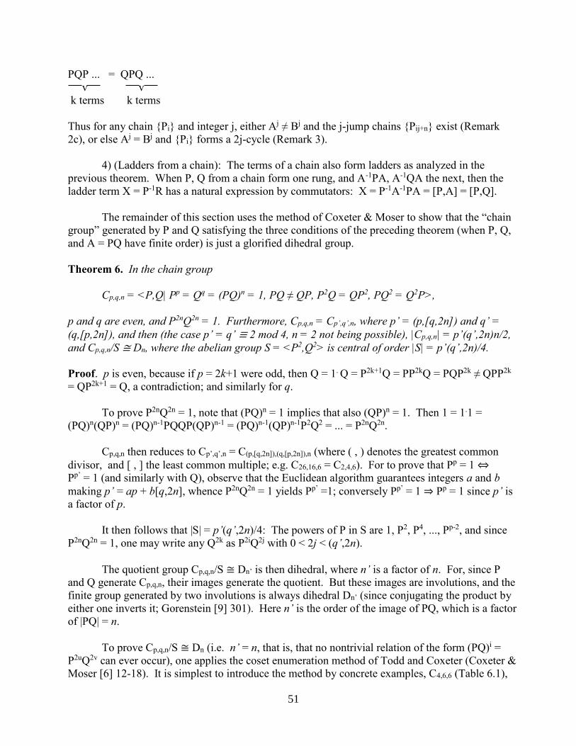
51

PQP ... = QPQ ...

v v

k terms k terms

Thus for any chain {Pi} and integer j, either Aj ≠ Bj and the j-jump chains {Pij+n} exist (Remark

2c), or else Aj = Bj and {Pi} forms a 2j-cycle (Remark 3).

4) (Ladders from a chain): The terms of a chain also form ladders as analyzed in the

previous theorem. When P, Q from a chain form one rung, and A-1PA, A-1QA the next, then the

ladder term X = P-1R has a natural expression by commutators: X = P-1A-1PA = [P,A] = [P,Q].

The remainder of this section uses the method of Coxeter & Moser to show that the “chain

group” generated by P and Q satisfying the three conditions of the preceding theorem (when P, Q,

and A = PQ have finite order) is just a glorified dihedral group.

Theorem 6. In the chain group

Cp,q,n = <P,Q| Pp = Qq = (PQ)n = 1, PQ ≠ QP, P2Q = QP2, PQ2 = Q2P>,

p and q are even, and P2nQ2n = 1. Furthermore, Cp,q,n = Cp’,q’,n, where p’ = (p,[q,2n]) and q’ =

(q,[p,2n]), and then (the case p’ = q’ ≡ 2 mod 4, n = 2 not being possible), |Cp,q,n| = p’(q’,2n)n/2,

and Cp,q,n/S ≅ Dn, where the abelian group S = <P2,Q2> is central of order |S| = p’(q’,2n)/4.

Proof. p is even, because if p = 2k+1 were odd, then Q = 1. Q = P2k+1Q = PP2kQ = PQP2k ≠ QPP2k

= QP2k+1 = Q, a contradiction; and similarly for q.

To prove P2nQ2n = 1, note that (PQ)n = 1 implies that also (QP)n = 1. Then 1 = 1.1 =

(PQ)n(QP)n = (PQ)n-1PQQP(QP)n-1 = (PQ)n-1(QP)n-1P2Q2 = ... = P2nQ2n.

Cp,q,n then reduces to Cp’,q’,n = C(p,[q,2n]),(q,[p,2n]),n (where ( , ) denotes the greatest common

divisor, and [ , ] the least common multiple; e.g. C26,16,6 = C2,4,6). For to prove that Pp = 1 ⇔

Pp’ = 1 (and similarly with Q), observe that the Euclidean algorithm guarantees integers a and b

making p’ = ap + b[q,2n], whence P2nQ2n = 1 yields Pp’ =1; conversely Pp’ = 1 ⇒ Pp = 1 since p’ is

a factor of p.

It then follows that |S| = p’(q’,2n)/4: The powers of P in S are 1, P2, P4, ..., Pp-2, and since

P2nQ2n = 1, one may write any Q2k as P2iQ2j with 0 < 2j < (q’,2n).

The quotient group Cp,q,n/S ≅ Dn’ is then dihedral, where n’ is a factor of n. For, since P

and Q generate Cp,q,n, their images generate the quotient. But these images are involutions, and the

finite group generated by two involutions is always dihedral Dn’ (since conjugating the product by

either one inverts it; Gorenstein [9] 301). Here n’ is the order of the image of PQ, which is a factor

of |PQ| = n.

To prove Cp,q,n/S ≅ Dn (i.e. n’ = n, that is, that no nontrivial relation of the form (PQ)i =

P2uQ2v can ever occur), one applies the coset enumeration method of Todd and Coxeter (Coxeter &

Moser [6] 12-18). It is simplest to introduce the method by concrete examples, C4,6,6 (Table 6.1),

52

and then C4,12,3 for odd n and “collapsing” (Table 6.2). The left-most column defines the cosets,

labeled by numbers and divided into b “blocks” of length q’ = |Q|, with the general formula:

kq’ + i = <P>(QP)kQi-1 0 < k < b-2, 1 < i < q’

The numbers in the table represent multiplication of the cosets by the group terms between

columns at the top (e.g. 2.P = 7). Sub-tables I, II, and V encode the relations P4 = Q6 = (PQ)6 = 1

by the fact that their left and right columns are the same; sub-tables III and IV encode P2Q = QP2

and PQ2 = Q2P by having their rightmost column match the column to the left of the dashed line.

Rows not containing “essentially different” products are suppressed, e.g. rows 2-6 of table II (since

2.Q, 3.Q, etc. are already in row 1).

The method of Coxeter & Moser consists of progressively filling in the table from the coset

definitions and other deduced relations; the method succeeds if the table “closes up,” as it does

after the 18th row of Table 1, leaving no gaps, inconsistencies, or undefined terms. The circled 7 2

in the first row of table III illustrates the process of deducing relations: Entries 1 1 1 2 1 2 7

follow directly from the coset definitions 1.P = 1, 1.Q = 2, and 2.P = 7. But the final circled entry

must be 2, since P2Q = QP2, thus implying the new relation 7.P = 2. This, together with the

definition 2.P = 7, then allows one to complete row 2 of table I. Once 14.P = 14 in table V halts the

generation of cosets, the circled deduced entries in tables III and IV allow one to complete the

entire table.

The completed coset table gives the order of the group: there are 18 cosets of 4 elements

each, so |C4,6,6| = 72.

In C4,6,6 the relation P2nQ2n = 1 deduced at the beginning of the Theorem is vacuous since

P12 = Q12 = 1. But otherwise the coset table collapses to a much shorter length, because each block

has not q’ cosets, but only (q’,2n), repeating thereafter. Table 2 illustrates the shortened coset table

of C4,12,3 (retaining the coset numbering from the “uncollapsed” case). C4,12,3 also illustrates the

special features of the top block in a coset table with odd n: table I is empty, the top block has only

half as many cosets as the rest, and its table II consequently cycles through its cosets twice as often.

In the general case, periodicities apparent in the examples simplify the analysis

considerably. Observe, first, that P2 = 1 on cosets. For by definition 1.P = 1, so also 1.P2 = 1; and a

succeeding coset k+1 has the form either k.P (inductively unaffected by P2), or k.Q (inductively

unaffected by P2 since QP2 = P2Q). Hence the columns of table I (showing coset multiplication by

P) repeat in pairs; and table III holds trivially and will always “close up” if table I does.

Furthermore, each row beyond the first two in a block is the Q2-translate of the row two

above it. This is trivially true for the leftmost column in each sub-table, which is just the cosets in

ascending order. Columns thereafter arise through multiplication by P or Q at the top of the table,

and Q2P = PQ2 (by definition), and Q2Q = QQ2 (trivially).

In consequence, the entries in block k+1 (1<k<b-1) are those of block k shifted forward by

q. For table V has entries only in the first block, while table II, with entries only in the first row of

each block, has the required shift by definition. The other sub-tables, by the above discussion,

need be checked only in the first two rows of each block. In table I, by the discussion, one need

check only the first two columns. Only even rows appear in these blocks (cf. sample Table 6.1).

53

The assertion is trivial for column 1, which is just the even numbered cosets; and the row 2 column

2 entry in the kth block is by definition always the first coset in the k+1st block, yielding the

required pattern. Tables III and IV follow because multiplication by P has the desired shift (via

table I) and changes the block by at most 1, and P2 = 1, while multiplication by Q has the desired

shift (via table II) and leaves the block unchanged.

Since applying PQ repetitively moves a coset steadily first up the blocks, then back down

(table V), the constraint (PQ)n = 1 dictates that the number of blocks is b = n/2. (When n is odd,

the top block is only half-length, as in Table 6.2.) In more detail, the values 1.(PQ)i in the left half

of the first row of table V are 2+(i-1)q’ for i = 1,2,..., while in the right half the values 1.(PQ)-iP are

2+(i-1)q’ - 2i for i = 1,2,... (Here 2+(i-1)q’ is always the second coset in block i, and -2i denotes an

offset taken modulo (q’,2n) within that block.) Hence when n is even, the table V row will close

up at its central meeting point i = b = n/2, at the product [2+(b-1)q’].P = 2+(b-1)q’ - 2b = 2+(b-1)q’

- n. The offset -n, congruent to n mod (q,2n) [which is 0 or (q’/2,n), depending as the 2-factor of q’

is < or > than the 2-factor of n], is consistent with P2 = 1, so allowing table I to close. When n is

odd, the central meeting point is [1 + (i-1)q’].Q = (i-1)q’ + (q’,2n) -2i+3 at i = (n+1)/2, an offset

mod (q’,2n) of 1-n. But Q, by definition in table II, offsets by 1. Hence, to make -n ≡ 0, the top

block must collapse by half, to a length of (q’,n) rather than (q’,2n). In summary, the requirement

that table V “close up” dictates: when n is even, a P-product allowing table I to close up in block b;

when n is odd, a Q-product allowing table II to close up provided that block b collapse to half size

as in the example Table 6.2.

The discussed periodicities reduce the analysis to checking just the first two rows of just the

first, second, and last (bth) blocks of the table; simple direct calculations now show that these

behave properly, so the coset table is consistent and “closes up.” In particular, Cp,q,n has n/2 blocks

each containing (q’,2n) cosets of p’ elements, proving that |Cp,q,n| = p’(q’,2n)n/2.

Since the coset table proof given so far was actually for the group defined by generators and

relations without the constraint PQ ≠ QP, it remains necessary, finally, to derive PQ ≠ QP from the

rest. P and Q cannot commute when n > 2 because they generate the nonabelian quotient Dn.

When n = 2, QP = P-1Q-1 (trivially) and 1 = P2nQ2n = P4Q4, whence QP = P-1(P4Q4)Q-1 = PQP2Q2,

proving PQ ≠ QP unless P2Q2 = 1. The latter does actually hold in the excluded case n = 2, p’ = q’

= 4k + 2, since then 1 = 1.1 = Pp’Qq’ = (P4Q4)kP2Q2 = P2Q2. But otherwise the coset table for Cp’,q’,2

closes up successfully after four rows, on account of first row coset products being either 2.P = 4,

3.P = 3, and 4.P = 2 in subtables V, IV, and III, respectively, or else 2.P = 2, 3.P = 3, and 4.P =4, the

generation of cosets 1 = <P>, 2 = 1.Q, 3 = 2.Q, 4 = 3.Q halting at 4 because Q4 = P-4 ∈ 1. The

relation P2Q2 = 1 (which would halt the cosets already at 2) thus is not true; hence PQ ≠ QP. ￭

54

Tab

le 6

.1. C

4,6

,6.

55

Tab

le 2

. C

4,1

2,3

T

ab

le 6

.2. C

4,1

2,3

.

56

Acknowledgments

I am grateful for the encouragement of my late advisor, Prof. Peter Hilton, at the beginning

of this project, and then for the opportunity to present my results in a series of talks at John Carroll

University in 2000, and at section meetings of the Mathematical Association of America held at

John Carroll University in 2004, and Cleveland State University in 2013. Technology trainer Ann

MacNamara, and other Cleveland Heights - University Heights public library staff, assisted my

struggles to PC-computer format my manuscript.

References

[1] Adams, Colin C. The Knot Book: An Elementary Introduction to the Mathematical Theory of

Knots, New York: W. H. Freeman, 1994.

[2] Bach, Anna Magdalena. Minuet in g, in: Notebook of Anna Magdalena Bach.

www.youtube.com/user/The Great Repertoire, 2015.

[3] Batten, Lynn Margaret, and Beutelspacher, Albrecht. The Theory of Finite Linear Spaces:

Combinatorics of Points and Lines, Cambridge: Cambridge University Press, 1993.

[4] Birkhoff, George D. Aesthetic Measure, Cambridge, MA: Harvard University Press, 1933.

[5] Borsuk, K. Multidimensional Analytic Geometry, Polish Scientific Publishers, 1969.

[6] Coxeter, H. S. M., and Moser, W. O. J. Generators and Relations for Discrete Groups, Berlin:

Springer-Verlag, 1957.

[7] Dickinson, Emily. "Safe in their Alabaster Chambers," In: The Complete Poems of Emily

Dickinson (Thomas H. Johnson, ed.), Boston: Little, Brown, and Co., 1960, No. 216, p.

100.

[8] Forte, Allen, and Gilbert, Steven E. Introduction to Schenkerian Analysis, New York: W. W.

Norton, 1982.

[9] Gorenstein, Daniel. Finite Groups, New York: Harper & Row, 1968.

[10] Haas, Robert. “Three-colorings of finite groups, or An algebra of nonequalities,”

Mathematics Magazine 63(4) (1990) 211-225.

[11] Hall, Marshall, Jr. The Theory of Groups, 2nd ed., New York: Chelsea, 1976.

[12] Harary, Frank, and Palmer, Edgar M. Graphical Enumeration, New York: Academic Press,

1973.

[13] Johnson, Thomas H. Emily Dickinson: An Interpretive Biography, Cambridge, Mass.: The

Belknap Press of Harvard Univ. Press, 1955, pp. 104-108.

[14] Kauffman, Louis H. “New invariants in the theory of knots,” American Math. Monthly 95

(1988) 195-242.

[15] Koshy, Thomas. Fibonacci and Lucas Numbers with Applications (Wiley-Interscience series,

Pure and Applied Mathematics), New York: John Wiley & Sons, 2001.

[16] Mu Qi. Six Persimmons, in: Sherman Lee, A History of Far Eastern Art (4th edition), New

York: Harry N. Abrams, Inc., 1982, p. 362.

[17] Sloane, Neil J. A. On-line Encyclopedia of Integer Sequences, http://www.research.att.com

/cgi-bin/access.cgi/as/njas/sequences/eismum.cgi.

[18] Waley, Arthur. An Introduction to the Study of Chinese Painting, London: Benn, 1923, p. 231.

Cited in: Sherman Lee, A History of Far Eastern Art (4th edition), New York: Harry N.

Abrams, Inc., 1982, p. 362.

[19] Weyl, Hermann. Symmetry, Princeton: Princeton Univ. Press, 1952.

http://www.research.att.com/

57

i Remark on nomenclature: The cographs in this article are quite distinct from the combinatorial

objects termed cographs. The term used in this article serves to recall 1) the familiar category-

theoretic duality, “reversing the arrows,” in Definition 1.1, and 2) the complete colored graphs in

Definition 1.2. I have used the term privately since 1980, in lectures in 2000, and in talks to local

section meetings of the MAA, in 2004 and 2013. Some evidence that cographs have not been

extensively studied under some other name is that the sequence 1, 3, 25, 1299, the number of

cographs on n points (Table 1.1), is not currently (2019) in the On-Line Encyclopedia of Integer

Sequences [17].

1 Cographsi Robert Haas 1. Introduction This article ... - arXiv

Documents

Transcript of 1 Cographsi Robert Haas 1. Introduction This article ... - arXiv