Modul ke:

Fakultas

Program Studi

Manajemen Persediaan

04 FEB

Manajemen

Penentuan Jumlah Persediaan dengan Metode Deterministik

Jenis Sistem Pengendalian Persediaan

• Sistem tempat persediaan tunggal – Bak/ papan diisi secara periodik, co: toko, pabrik – Disebut dengan sistem P

• Sistem tempat persediaan ganda – Tempat pesediaan dibagi2 yakni: persediaan yang akan dikeluarkan

dan persediaan yang masih disegel – Disebut dengan sistem Q

• Sistem kartu file – Terdapat 1 kartu untuk setiap item persediaan – Saat item terjual dan terisi kembali kartu korespondensi diperbaharui – Perpaduan sistem p dan sistem Q

• Sistem Komputer – Setiap item, transaksi penerimaan dicatat, berisikan keputusan dari

sistem P dan Q, peramalan permintaan, pemantauan kinerja persediaan

Periode Persediaan

• Persediaan periode tunggal

– Item yang akan di stok 1 kali dan setelah habis tidak akan dilakukan pemesanan kembali

• Persediaan periode ganda

– Persediaan yang akan dipertahankan keberadaannya dan akan dilakukan pemesanan kembali setelah dipergunakan/ terjual

– Dibagi menjadi 2 kategori yakni permintaan dependen dan independen

EOQ

• EOQ cocok diterapkan untuk item yang dibeli dari perusahaan lain

• EOQ banyak diterapkan untuk permintaan independen

• Digunakan untuk menentukan ukuran lot pemesanan dengan biaya yang paling optimal

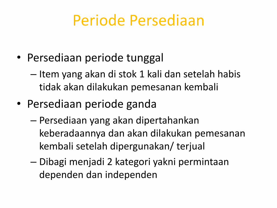
Syarat Model EOQ

• Tingkat penggunaan seragam dan diketahui • Harga item sama untuk setiap ukuran pemesanan • Semua pesanan dikirim pada waktu yang sama • Lead time konstan dan diketahui dengan baik • Item merupakan produk tunggal dan tidak ada

kaitannya dengan produk lain • Biaya penempatan dan penerimaan pesanan

diabaikan untuk sejumlah pesanan • Biaya item unit konstan dan tidak ada diskon

untuk pembelian dalam jumlah besar, tidak ada skala ekonomi dalam biaya penyimpanan item

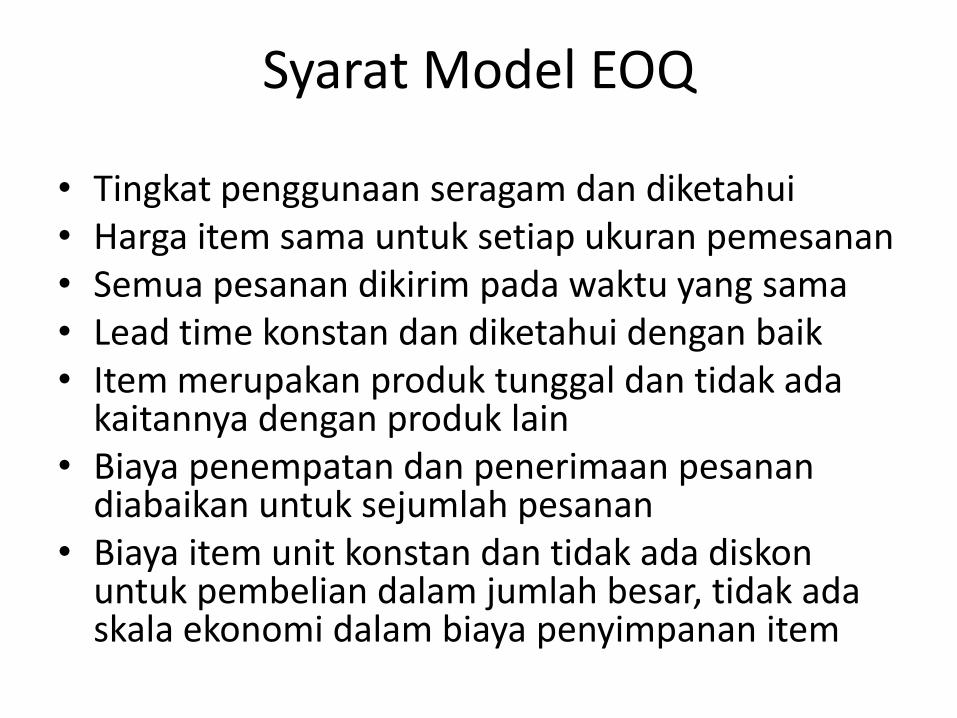
Inventories in the Supply Chain

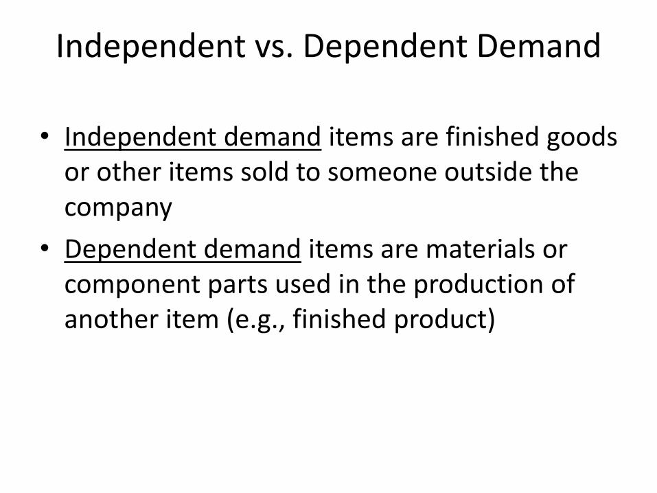
Independent vs. Dependent Demand

• Independent demand items are finished goods or other items sold to someone outside the company

• Dependent demand items are materials or component parts used in the production of another item (e.g., finished product)

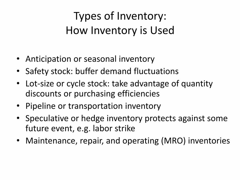
Types of Inventory: How Inventory is Used

• Anticipation or seasonal inventory

• Safety stock: buffer demand fluctuations

• Lot-size or cycle stock: take advantage of quantity discounts or purchasing efficiencies

• Pipeline or transportation inventory

• Speculative or hedge inventory protects against some future event, e.g. labor strike

• Maintenance, repair, and operating (MRO) inventories

Objectives of Inventory Management

• Provide acceptable level of customer service (on-time delivery)

• Allow cost-efficient operations

• Minimize inventory investment

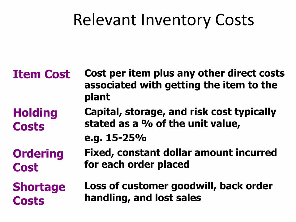
Relevant Inventory Costs

Item Cost Cost per item plus any other direct costs associated with getting the item to the plant

Holding Costs

Capital, storage, and risk cost typically stated as a % of the unit value,

e.g. 15-25%

Ordering Cost

Fixed, constant dollar amount incurred for each order placed

Shortage Costs

Loss of customer goodwill, back order handling, and lost sales

Order Quantity Strategies

Lot-for-lot Order exactly what is needed for the next period

Fixed-order quantity

Order a predetermined amount each time an order is placed

Min-max system

When on-hand inventory falls below a predetermined minimum level, order enough to refill up to maximum level

Order n periods

Order enough to satisfy demand for the next n periods

Examples of Ordering Approaches

Lot for Lot Example

1 2 3 4 5 6 7 8

Requirements 70 70 65 60 55 85 75 85

Projected-on-Hand (30) 0 0 0 0 0 0 0

Order Placement 40 70 65 60 55 85 75 85

Fixed Order Quantity Example with Order Quantity of 200

1 2 3 4 5 6 7 8

Requirements 70 70 65 60 55 85 75 85

Projected-on-Hand (30) 160 90 25 165 110 25 150 65

Order Placement 200 200 200

Min-Max Example with min.= 50 and max.= 250 units

1 2 3 4 5 6 7 8

Requirements 70 70 65 60 55 85 75 85

Projected-on-Hand (30) 180 110 185 125 70 165 90 165

Order Placement 220 140 180 160

Order n Periods with n = 3 periods

1 2 3 4 5 6 7 8

Requirements 70 70 65 60 55 85 75 85

Projected-on-Hand (30) 135 65 0 140 85 0 85 0

Order Placement 175 200 160

Three Mathematical Models for Determining Order Quantity

• Economic Order Quantity (EOQ or Q System)

– An optimizing method used for determining order quantity and reorder points

– Part of continuous review system which tracks on-hand inventory each time a withdrawal is made

• Economic Production Quantity (EPQ)

– A model that allows for incremental product delivery

• Quantity Discount Model

– Modifies the EOQ process to consider cases where quantity discounts are available

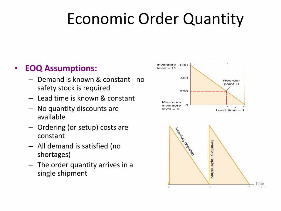
Economic Order Quantity

• EOQ Assumptions: – Demand is known & constant - no

safety stock is required

– Lead time is known & constant

– No quantity discounts are available

– Ordering (or setup) costs are constant

– All demand is satisfied (no shortages)

– The order quantity arrives in a single shipment

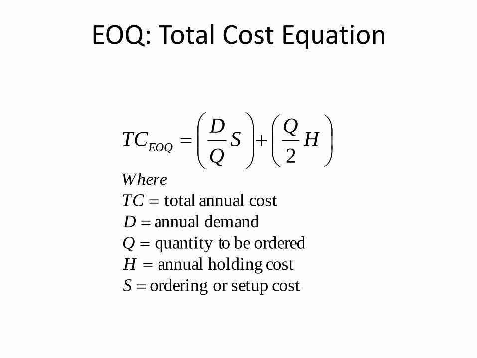
EOQ: Total Cost Equation

cost setupor ordering

cost holding annual

ordered be oquantity t

demand annual

cost annual total

2

S

H

Q

D

TC

Where

HQ

SQ

DTCEOQ

EOQ Total Costs

Total annual costs = annual ordering costs + annual holding costs

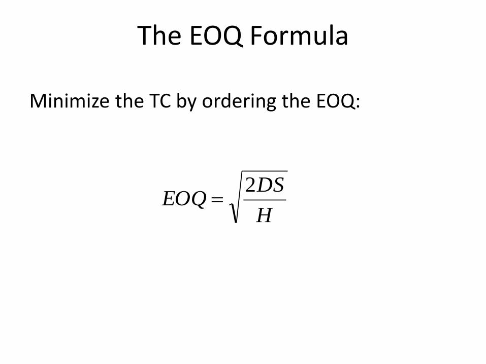
The EOQ Formula

Minimize the TC by ordering the EOQ:

H

DSEOQ

2

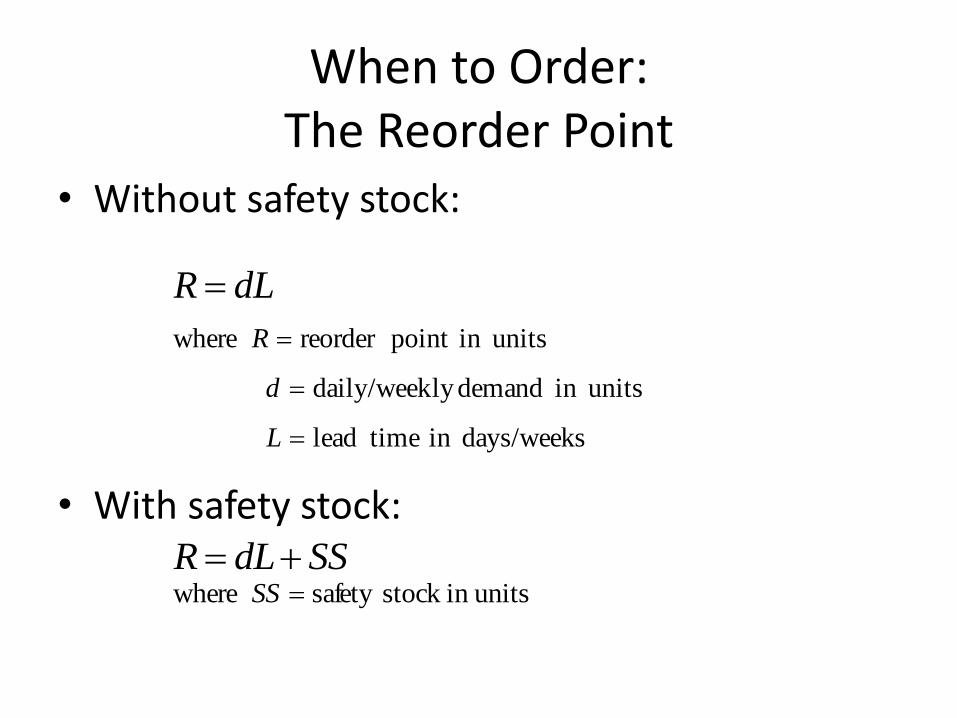
When to Order: The Reorder Point

• Without safety stock:

• With safety stock:

days/weeksintimelead

unitsindemandlydaily/week

unitsinpointreorderwhere

L

d

R

dLR

unitsin stock safety where

SS

SSdLR

ROP = LxD

Receive

order

Time

Inven

tory

Order

Quantity

Q

Place

order

Lead Time

Reorder

Point

(ROP)

If demand is known exactly, place an order when inventory equals demand during lead time.

D: demand per period L: Lead time in periods

Q: When shall we order?

A: When inventory = ROP

Q: How much shall we order?

A: Q = EOQ

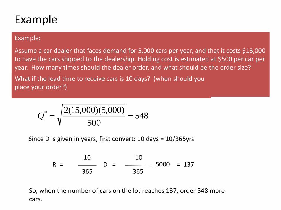
Example

10

365 D = R =

10

365 5000 = 137

So, when the number of cars on the lot reaches 137, order 548 more cars.

Since D is given in years, first convert: 10 days = 10/365yrs

Example:

Assume a car dealer that faces demand for 5,000 cars per year, and that it costs $15,000 to have the cars shipped to the dealership. Holding cost is estimated at $500 per car per year. How many times should the dealer order, and what should be the order size?

What if the lead time to receive cars is 10 days? (when should you place your order?)

548500

)000,5)(000,15(2* Q

TimeTime

Inventory Inventory

LevelLevel

OrderOrder

QuantityQuantity

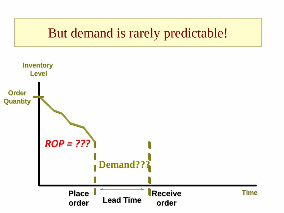
But demand is rarely predictable!

Demand???

Receive

order

Place

order Lead Time

ROP = ???

XX

Inventory at time of receipt

Receive Receive

orderorder

TimeTime

Inventory Inventory

LevelLevel

OrderOrder

QuantityQuantity

PlacePlace

orderorder

Lead TimeLead Time

Actual Demand < Expected Demand

ROP

Lead Time Demand

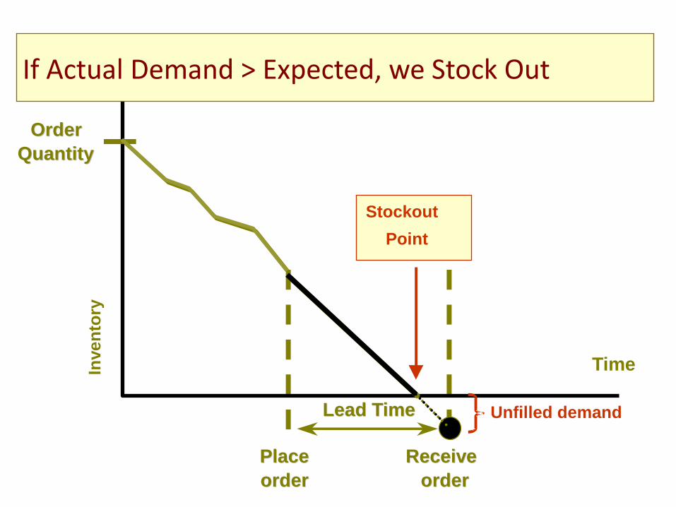
Stockout

Point

Unfilled demand

Receive Receive

order order

Time Inven

tory

Order Order

Quantity Quantity

Place Place

order order

Lead Time Lead Time

If Actual Demand > Expected, we Stock Out

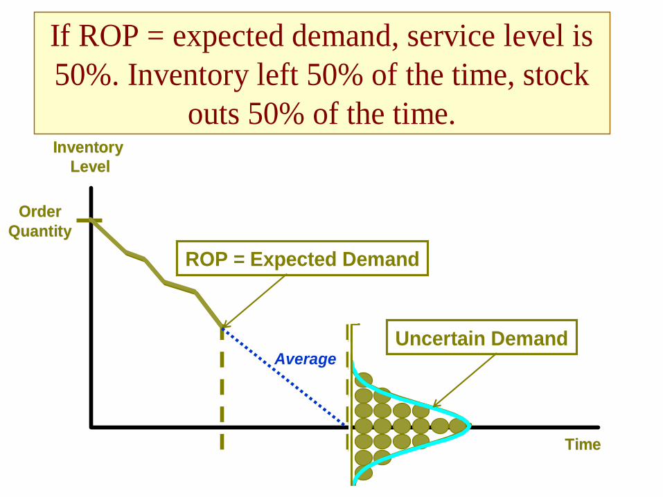
ROP = Expected Demand

Average

TimeTime

Inventory Inventory

LevelLevel

OrderOrder

QuantityQuantity

If ROP = expected demand, service level is

50%. Inventory left 50% of the time, stock

outs 50% of the time.

Uncertain Demand

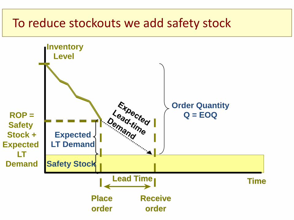
To reduce stockouts we add safety stock

Receive Receive

order order

Time Time

Place Place

order order

Lead Time Lead Time

Inventory Level

ROP =

Safety

Stock +

Expected

LT Demand

Order Quantity Q = EOQ

Expected LT Demand

Safety Stock

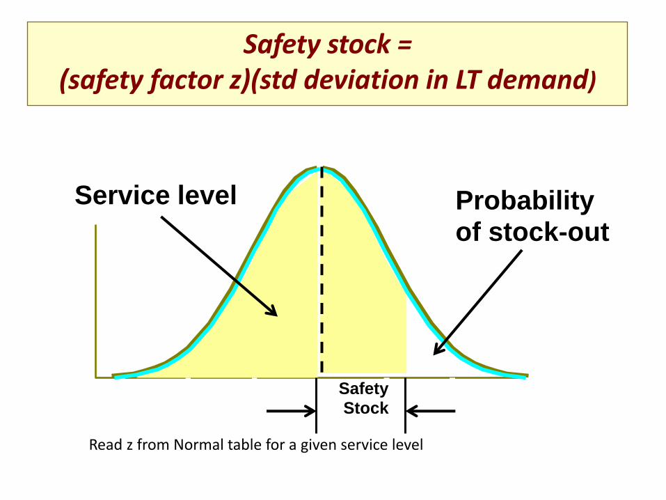
Service level

Safety

Stock

Probability of stock-out

Decide what Service Level you want to provide (Service level = probability of NOT stocking out)

Service level

Safety

Stock

Probability of stock-out

Safety stock = (safety factor z)(std deviation in LT demand)

Read z from Normal table for a given service level

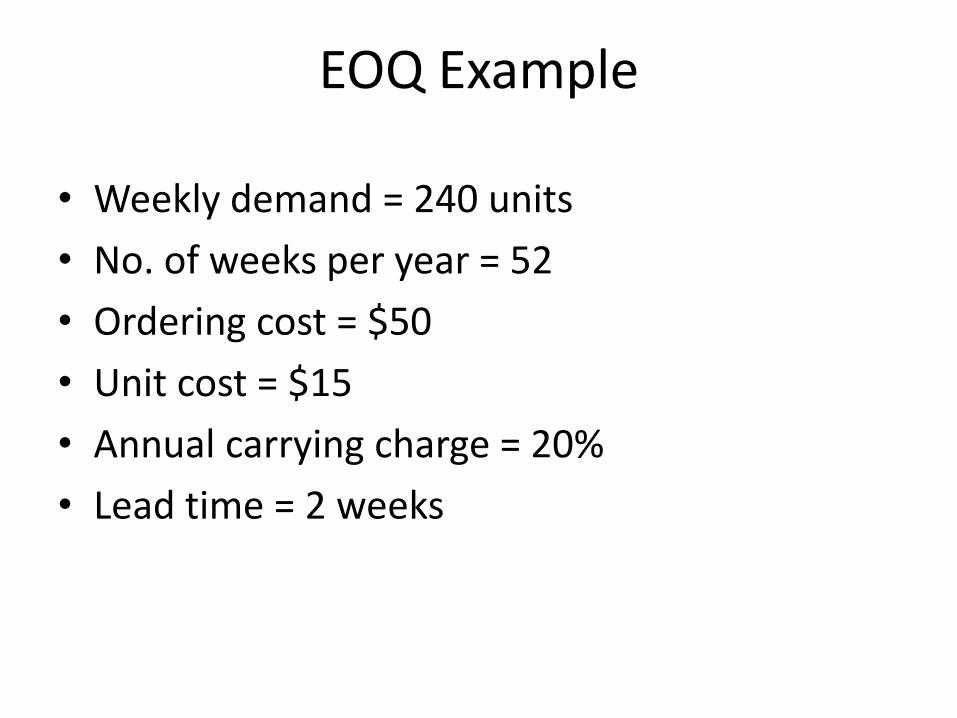
EOQ Example

• Weekly demand = 240 units

• No. of weeks per year = 52

• Ordering cost = $50

• Unit cost = $15

• Annual carrying charge = 20%

• Lead time = 2 weeks

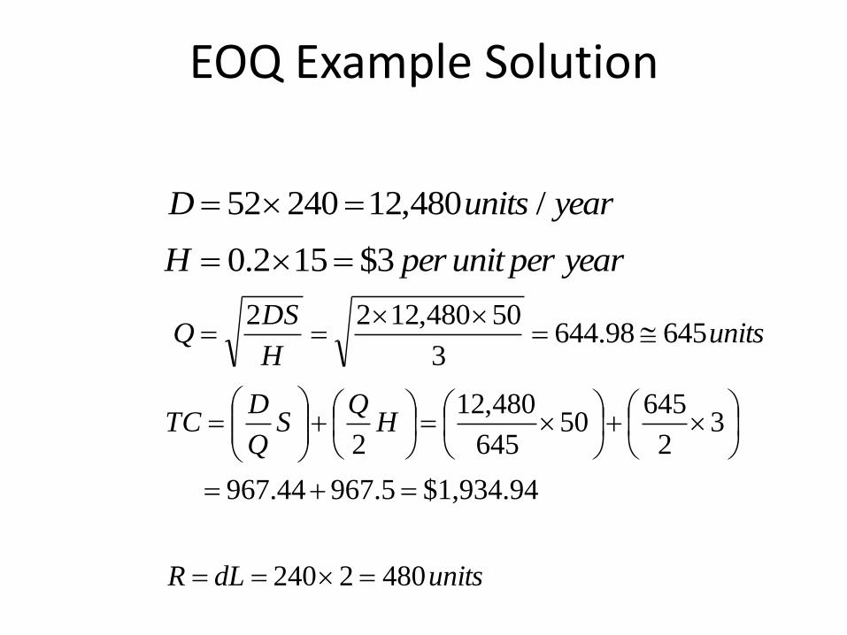
EOQ Example Solution

yearunitsD /480,1224052

yearperunitperH 3$152.0

unitsH

DSQ 64598.644

3

50480,1222

unitsdLR

HQ

SQ

DTC

4802240

$1,934.945.96744.967

32

64550

645

480,12

2

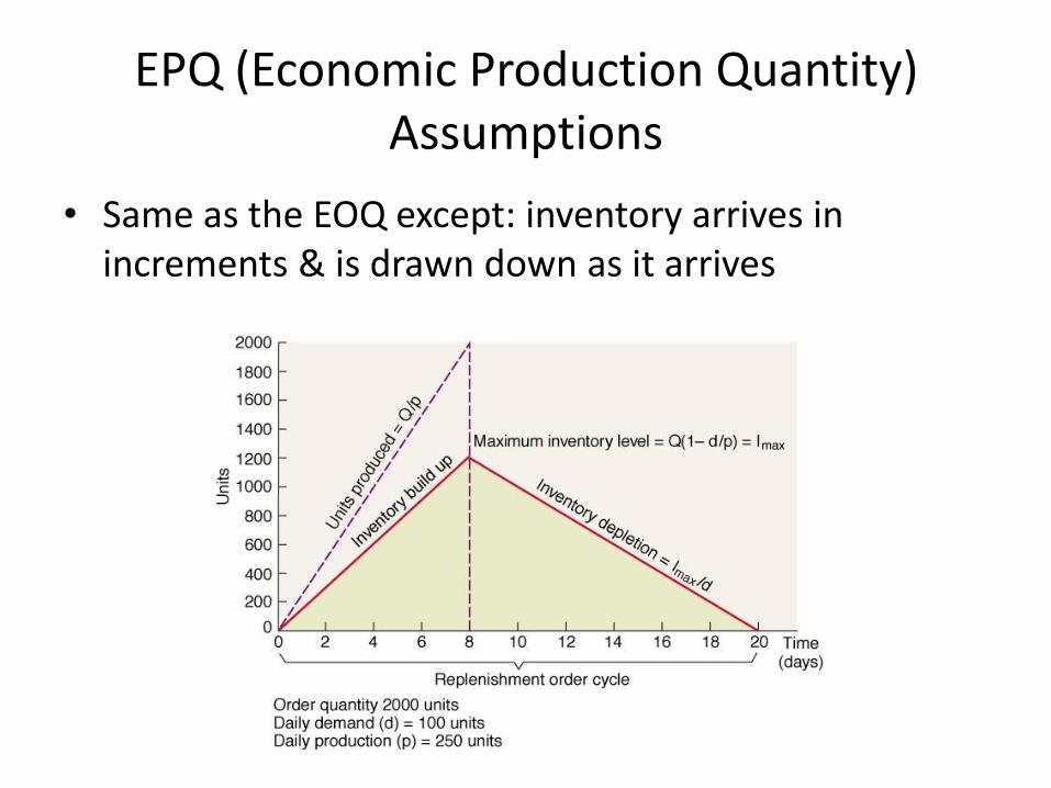
EPQ (Economic Production Quantity) Assumptions

• Same as the EOQ except: inventory arrives in increments & is drawn down as it arrives

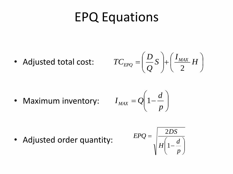
EPQ Equations

• Adjusted total cost:

• Maximum inventory:

• Adjusted order quantity:

H

IS

Q

DTC MAX

EPQ2

p

dQIMAX 1

p

dH

DSEPQ

1

2

EPQ Example

• Annual demand = 18,000 units

• Production rate = 2500 units/month

• Setup cost = $800

• Annual holding cost = $18 per unit

• Lead time = 5 days

• No. of operating days per month = 20

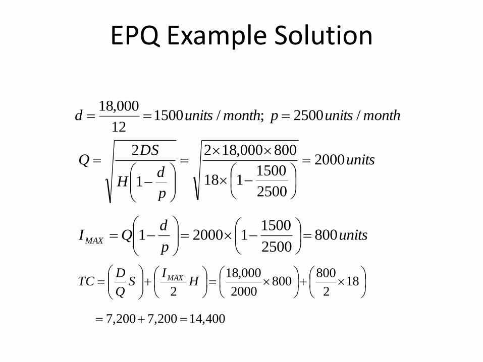
EPQ Example Solution

monthunitspmonthunitsd /2500;/150012

000,18

units

p

dH

DSQ 2000

2500

1500118

800000,182

1

2

unitsp

dQIMAX 800

2500

1500120001

400,14200,7200,7

182

800800

2000

000,18

2

H

IS

Q

DTC MAX

EPQ Example Solution (cont.)

• The reorder point:

• With safety stock of 200 units:

unitsSSdLR 575200520

1500

unitsdLR 375520

1500

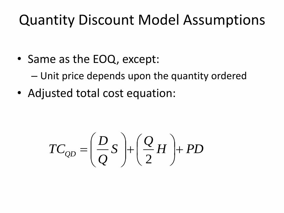
Quantity Discount Model Assumptions

• Same as the EOQ, except:

– Unit price depends upon the quantity ordered

• Adjusted total cost equation:

PDHQ

SQ

DTCQD

2

Daftar Pustaka

• Richardus Eko Indrajit, (2005), Manajemen Persediaan, Grasindo, Jakarta

• Heizer Jay, B.Rander, (206), Manajemen Operasi, Salemba Empat, Jakarta

• Hani handoko, (2002), Manajemen Produksi dan Operasi, BPFE, Yogyakarta

• Siswanto, (2005), Riset Operasi, Erlangga, Jakarta

• M. Syamsul Ma’arif, (2003), Manajemen Operasi, Grasindo, Jakarta

• Sofyan Assauri, (2001), Manajemen Operasi, BPFE, Jakarta

• Martinich, (2003), Operation Manaement, Prenice hall, New Yory

Terima Kasih