Dong Zhang's project

Modified Kolmogorov-Smirnov

Goodness-of-Fit Test for GARCH

Models with Mixture of Normal

Innovations

Dong Zhang

Supervisor: Hao Yu

Department of Statistical and Actuarial Sciences

University of Western Ontario

August 8, 2013

Abstract

In many financial fields, the GARCH model plays an important

role in modeling the return rates of securities, such as stocks. In the

meantime, the Kolmogorov-Smirnov (KS) test is one of the common

way to test whether the innovation is from a specific distribution. In

this project we use the modified KS statistic to test if the innovation

of a GARCH model is from a mixture of normal distribution instead

of a standard normal distribution. Simulation study is conducted

to study the size and power of the KS and the modified KS tests.

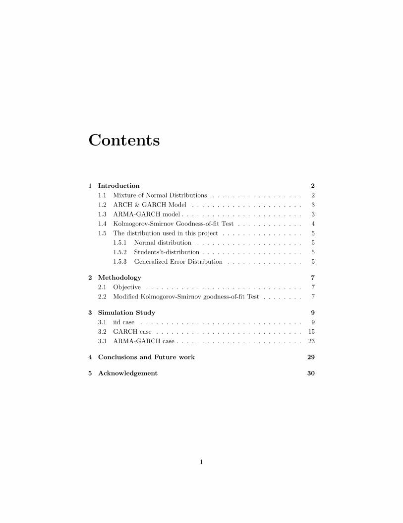
Contents

1 Introduction 2

1.1 Mixture of Normal Distributions . . . . . . . . . . . . . . . . . . 2

1.2 ARCH & GARCH Model . . . . . . . . . . . . . . . . . . . . . . 3

1.3 ARMA-GARCH model . . . . . . . . . . . . . . . . . . . . . . . . 3

1.4 Kolmogorov-Smirnov Goodness-of-fit Test . . . . . . . . . . . . . 4

1.5 The distribution used in this project . . . . . . . . . . . . . . . . 5

1.5.1 Normal distribution . . . . . . . . . . . . . . . . . . . . . 5

1.5.2 Students’t-distribution . . . . . . . . . . . . . . . . . . . . 5

1.5.3 Generalized Error Distribution . . . . . . . . . . . . . . . 5

2 Methodology 7

2.1 Objective . . . . . . . . . . . . . . . . . . . . . . . . . . . . . . . 7

2.2 Modified Kolmogorov-Smirnov goodness-of-fit Test . . . . . . . . 7

3 Simulation Study 9

3.1 iid case . . . . . . . . . . . . . . . . . . . . . . . . . . . . . . . . 9

3.2 GARCH case . . . . . . . . . . . . . . . . . . . . . . . . . . . . . 15

3.3 ARMA-GARCH case . . . . . . . . . . . . . . . . . . . . . . . . . 23

4 Conclusions and Future work 29

5 Acknowledgement 30

1

Chapter 1

Introduction

1.1 Mixture of Normal Distributions

In probability and statistics, a mixture distribution is the probability distribu-

tion of a random variable whose values can be interpreted as being derived in the

following way from an underlying set of other random variables: In cases where

each of the underlying random variables is continuous, the outcome variable will

also be continuous and its probability density function is sometimes referred to

as a mixture density. The cumulative distribution function (and the probability

density function if it exists) can be expressed as a convex combination (i.e. a

weighted sum, with non-negative weights that sum to 1) of other distribution

functions and density functions. The individual distributions that are combined

to form the mixture distribution are called the mixture components, and the

probabilities (or weights) associated with each component are called the mix-

ture weights.

In this project, I use the mixture of two independent normal distributions. In

other words,we have a random variable X and the observations are X1, . . . , Xn.

Then we can see

X ∼ N(µ1, σ21) with probability λ,

and

X ∼ N(µ2, σ22) with probability 1− λ.

2

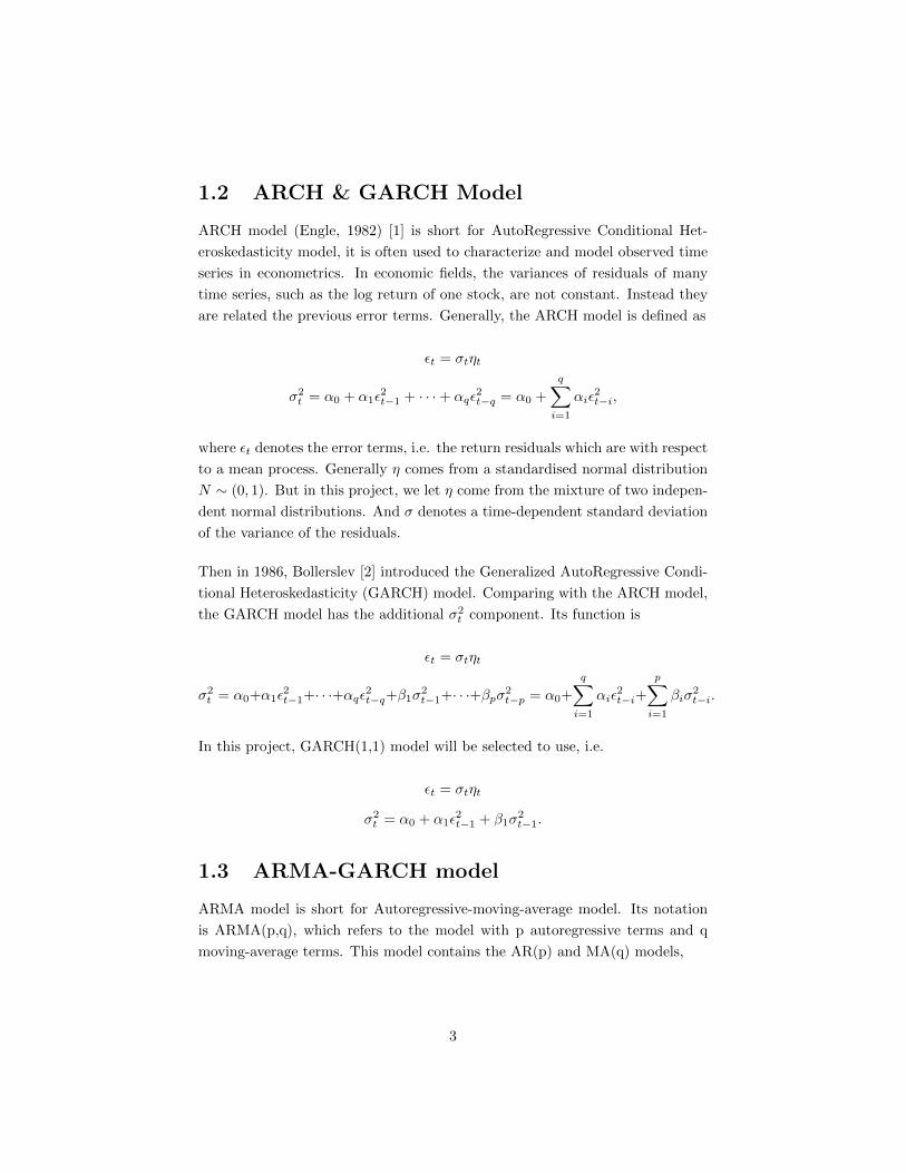
1.2 ARCH & GARCH Model

ARCH model (Engle, 1982) [1] is short for AutoRegressive Conditional Het-

eroskedasticity model, it is often used to characterize and model observed time

series in econometrics. In economic fields, the variances of residuals of many

time series, such as the log return of one stock, are not constant. Instead they

are related the previous error terms. Generally, the ARCH model is defined as

εt = σtηt

σ2t = α0 + α1ε

2t−1 + · · ·+ αqε

2t−q = α0 +

q∑i=1

αiε2t−i,

where εt denotes the error terms, i.e. the return residuals which are with respect

to a mean process. Generally η comes from a standardised normal distribution

N ∼ (0, 1). But in this project, we let η come from the mixture of two indepen-

dent normal distributions. And σ denotes a time-dependent standard deviation

of the variance of the residuals.

Then in 1986, Bollerslev [2] introduced the Generalized AutoRegressive Condi-

tional Heteroskedasticity (GARCH) model. Comparing with the ARCH model,

the GARCH model has the additional σ2t component. Its function is

εt = σtηt

σ2t = α0+α1ε

2t−1+· · ·+αqε2t−q+β1σ2

t−1+· · ·+βpσ2t−p = α0+

q∑i=1

αiε2t−i+

p∑i=1

βiσ2t−i.

In this project, GARCH(1,1) model will be selected to use, i.e.

εt = σtηt

σ2t = α0 + α1ε

2t−1 + β1σ

2t−1.

1.3 ARMA-GARCH model

ARMA model is short for Autoregressive-moving-average model. Its notation

is ARMA(p,q), which refers to the model with p autoregressive terms and q

moving-average terms. This model contains the AR(p) and MA(q) models,

3

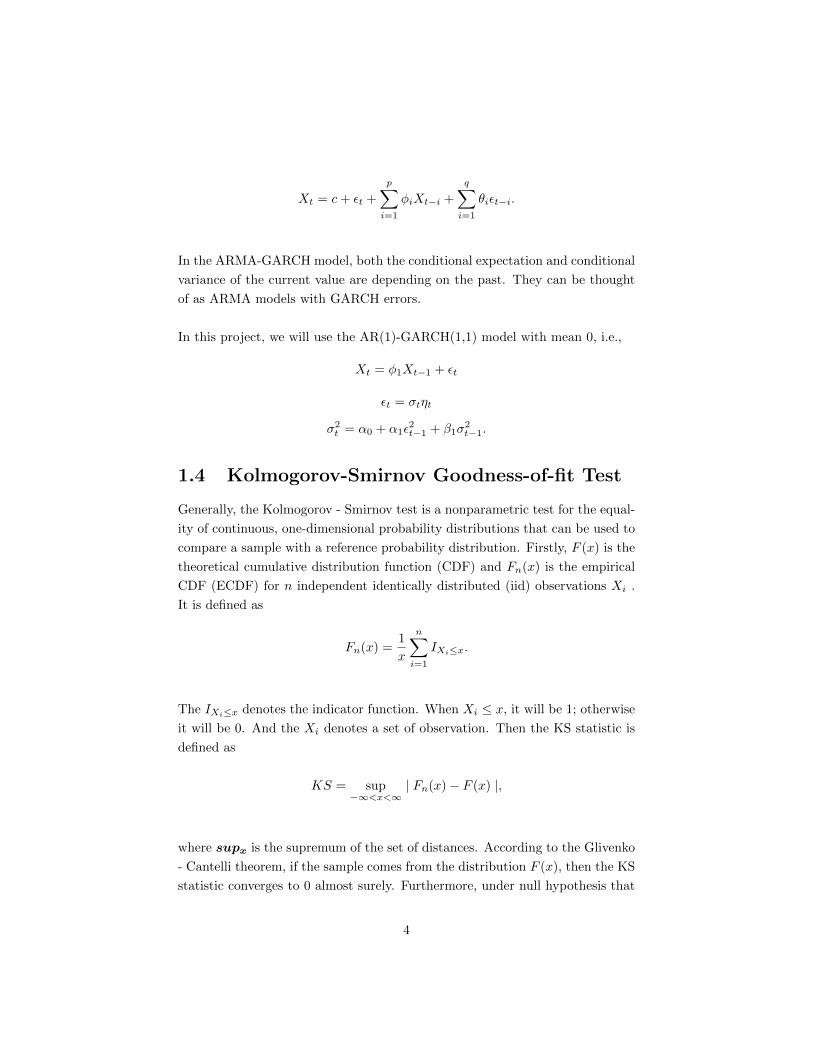
Xt = c+ εt +

p∑i=1

φiXt−i +

q∑i=1

θiεt−i.

In the ARMA-GARCH model, both the conditional expectation and conditional

variance of the current value are depending on the past. They can be thought

of as ARMA models with GARCH errors.

In this project, we will use the AR(1)-GARCH(1,1) model with mean 0, i.e.,

Xt = φ1Xt−1 + εt

εt = σtηt

σ2t = α0 + α1ε

2t−1 + β1σ

2t−1.

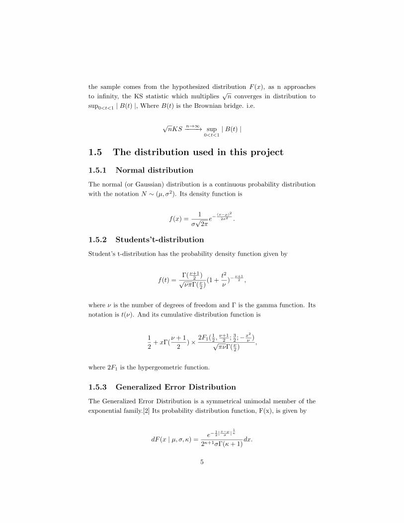
1.4 Kolmogorov-Smirnov Goodness-of-fit Test

Generally, the Kolmogorov - Smirnov test is a nonparametric test for the equal-

ity of continuous, one-dimensional probability distributions that can be used to

compare a sample with a reference probability distribution. Firstly, F (x) is the

theoretical cumulative distribution function (CDF) and Fn(x) is the empirical

CDF (ECDF) for n independent identically distributed (iid) observations Xi .

It is defined as

Fn(x) =1

x

n∑i=1

IXi≤x.

The IXi≤x denotes the indicator function. When Xi ≤ x, it will be 1; otherwise

it will be 0. And the Xi denotes a set of observation. Then the KS statistic is

defined as

KS = sup−∞<x<∞

| Fn(x)− F (x) |,

where supx is the supremum of the set of distances. According to the Glivenko

- Cantelli theorem, if the sample comes from the distribution F (x), then the KS

statistic converges to 0 almost surely. Furthermore, under null hypothesis that

4

the sample comes from the hypothesized distribution F (x), as n approaches

to infinity, the KS statistic which multiplies√n converges in distribution to

sup0<t<1 | B(t) |, Where B(t) is the Brownian bridge. i.e.

√nKS

n→∞−−−−→ sup0<t<1

| B(t) |

1.5 The distribution used in this project

1.5.1 Normal distribution

The normal (or Gaussian) distribution is a continuous probability distribution

with the notation N ∼ (µ, σ2). Its density function is

f(x) =1

σ√

2πe−

(x−µ)2

2σ2 .

1.5.2 Students’t-distribution

Student’s t-distribution has the probability density function given by

f(t) =Γ(ν+1

2 )√νπΓ(ν2 )

(1 +t2

ν)−

ν+12 ,

where ν is the number of degrees of freedom and Γ is the gamma function. Its

notation is t(ν). And its cumulative distribution function is

1

2+ xΓ(

ν + 1

2)×

2F1( 12 ,

ν+12 ; 3

2 ;−x2

ν )√πνΓ(ν2 )

,

where 2F1 is the hypergeometric function.

1.5.3 Generalized Error Distribution

The Generalized Error Distribution is a symmetrical unimodal member of the

exponential family.[2] Its probability distribution function, F(x), is given by

dF (x | µ, σ, κ) =e−

12 |x−µσ |

1κ

2κ+1σΓ(κ+ 1)dx.

5

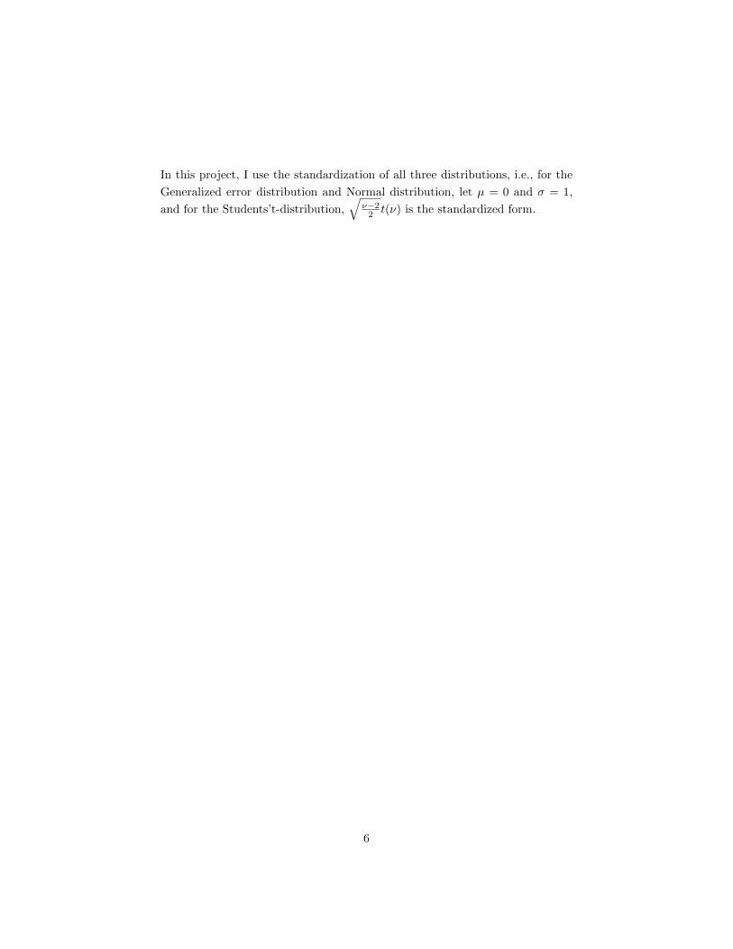
In this project, I use the standardization of all three distributions, i.e., for the

Generalized error distribution and Normal distribution, let µ = 0 and σ = 1,

and for the Students’t-distribution,√

ν−22 t(ν) is the standardized form.

6

Chapter 2

Methodology

2.1 Objective

The main objective of this project is to test if the innovation of GARCH model

comes from the mixture of normal distribution, which is

η ∼MN(λ, µ1, σ21 , µ2, σ

22).

In order to complete this objective, in this project the one of the most common

goodness-of-fit tests – KS test will be used. In addition to the original KS

test, the modified KS (MKS) test will also be introduced. After getting the

two tests, we can conduct the simulation study for different sample sizes and

three alternative distributions - Normal distribution, Student’s t-distribution

and Generalized error distribution to calculate the rejection rete(power).

2.2 Modified Kolmogorov-Smirnov goodness-of-

fit Test

According to the study of J. Kawczak, R. Kulperger, and H. Yu [2], the original

KS test will have undesired power and size when dealing with the innovation

of GARCH model with mean included. Furthermore, Yu [3] has shown that

the modified KS test is valid for GARCH residuals regardless of whether the

mean is included or not. So here we introduce the modified KS test in order to

overcome this problem. In order to get the modified one, we should first define

7

the standardization for the data(residuals), i.e. for a process {ηt, t = 1 · · ·n}

η̇t =ηt − η̄σηt

,

where η̇t denotes the standardized ηt, η̄ denotes the sample mean of ηt, σηt

denotes the standard deviation of ηt. After that, we can calculate the modified

KS statistic, i.e.

MKS = sup−∞<x<∞

| F η̇tn (x)− F (x) | .

Here Yu [3] has also shown that, as the sample size n increases to infinity, under

the null hypothesis, the empirical process based on the standardized residuals

will converge to the empirical process based on the standardized innovations, by

assuming the parameter estimator being√n consistent. Therefore, the model

parameters under the null hypothesis will not be influenced by the distribution

of modified KS test statistic. Based on this result, we can calculate the critical

value of the modified KS test by simulating the empirical process based on the

standardized innovations. Then use the similar method as we calculate the KS

statistic, we can get the modified KS statistic. And if the test statistic is too

large, we will reject the null hypothesis.

8

Chapter 3

Simulation Study

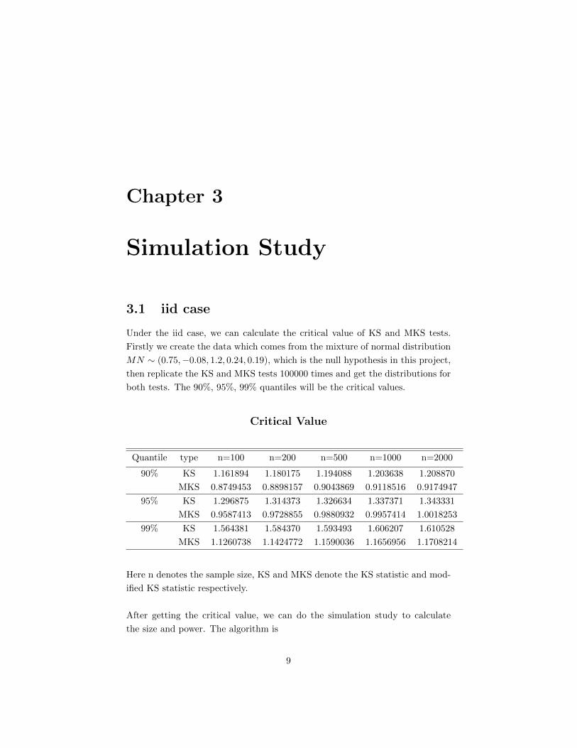
3.1 iid case

Under the iid case, we can calculate the critical value of KS and MKS tests.

Firstly we create the data which comes from the mixture of normal distribution

MN ∼ (0.75,−0.08, 1.2, 0.24, 0.19), which is the null hypothesis in this project,

then replicate the KS and MKS tests 100000 times and get the distributions for

both tests. The 90%, 95%, 99% quantiles will be the critical values.

Critical Value

Quantile type n=100 n=200 n=500 n=1000 n=2000

90% KS 1.161894 1.180175 1.194088 1.203638 1.208870

MKS 0.8749453 0.8898157 0.9043869 0.9118516 0.9174947

95% KS 1.296875 1.314373 1.326634 1.337371 1.343331

MKS 0.9587413 0.9728855 0.9880932 0.9957414 1.0018253

99% KS 1.564381 1.584370 1.593493 1.606207 1.610528

MKS 1.1260738 1.1424772 1.1590036 1.1656956 1.1708214

Here n denotes the sample size, KS and MKS denote the KS statistic and mod-

ified KS statistic respectively.

After getting the critical value, we can do the simulation study to calculate

the size and power. The algorithm is

9

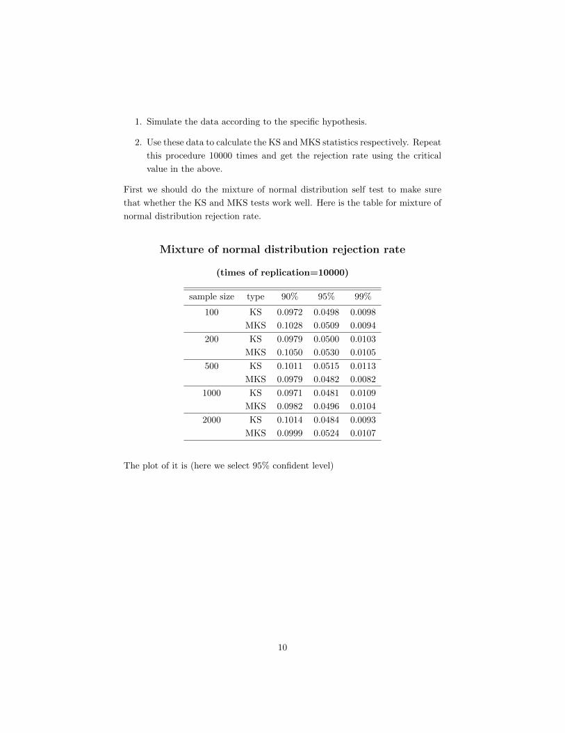
1. Simulate the data according to the specific hypothesis.

2. Use these data to calculate the KS and MKS statistics respectively. Repeat

this procedure 10000 times and get the rejection rate using the critical

value in the above.

First we should do the mixture of normal distribution self test to make sure

that whether the KS and MKS tests work well. Here is the table for mixture of

normal distribution rejection rate.

Mixture of normal distribution rejection rate

(times of replication=10000)

sample size type 90% 95% 99%

100 KS 0.0972 0.0498 0.0098

MKS 0.1028 0.0509 0.0094

200 KS 0.0979 0.0500 0.0103

MKS 0.1050 0.0530 0.0105

500 KS 0.1011 0.0515 0.0113

MKS 0.0979 0.0482 0.0082

1000 KS 0.0971 0.0481 0.0109

MKS 0.0982 0.0496 0.0104

2000 KS 0.1014 0.0484 0.0093

MKS 0.0999 0.0524 0.0107

The plot of it is (here we select 95% confident level)

10

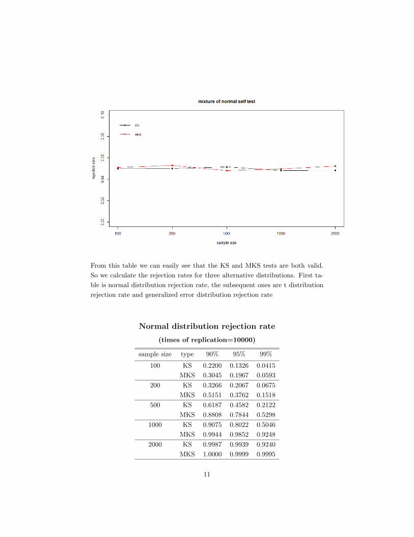
From this table we can easily see that the KS and MKS tests are both valid.

So we calculate the rejection rates for three alternative distributions. First ta-

ble is normal distribution rejection rate, the subsequent ones are t distribution

rejection rate and generalized error distribution rejection rate

Normal distribution rejection rate



100 KS 0.2200 0.1326 0.0415

MKS 0.3045 0.1967 0.0593

200 KS 0.3266 0.2067 0.0675

MKS 0.5151 0.3762 0.1518

500 KS 0.6187 0.4582 0.2122

MKS 0.8808 0.7844 0.5298

1000 KS 0.9075 0.8022 0.5046

MKS 0.9944 0.9852 0.9248

2000 KS 0.9987 0.9939 0.9240

MKS 1.0000 0.9999 0.9995

11

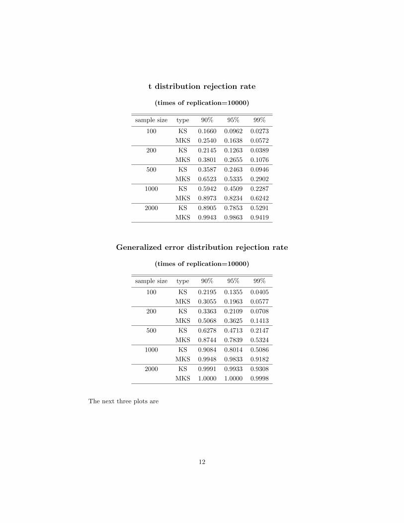
t distribution rejection rate



100 KS 0.1660 0.0962 0.0273

MKS 0.2540 0.1638 0.0572

200 KS 0.2145 0.1263 0.0389

MKS 0.3801 0.2655 0.1076

500 KS 0.3587 0.2463 0.0946

MKS 0.6523 0.5335 0.2902

1000 KS 0.5942 0.4509 0.2287

MKS 0.8973 0.8234 0.6242

2000 KS 0.8905 0.7853 0.5291

MKS 0.9943 0.9863 0.9419

Generalized error distribution rejection rate



100 KS 0.2195 0.1355 0.0405

MKS 0.3055 0.1963 0.0577

200 KS 0.3363 0.2109 0.0708

MKS 0.5068 0.3625 0.1413

500 KS 0.6278 0.4713 0.2147

MKS 0.8744 0.7839 0.5324

1000 KS 0.9084 0.8014 0.5086

MKS 0.9948 0.9833 0.9182

2000 KS 0.9991 0.9933 0.9308

MKS 1.0000 1.0000 0.9998

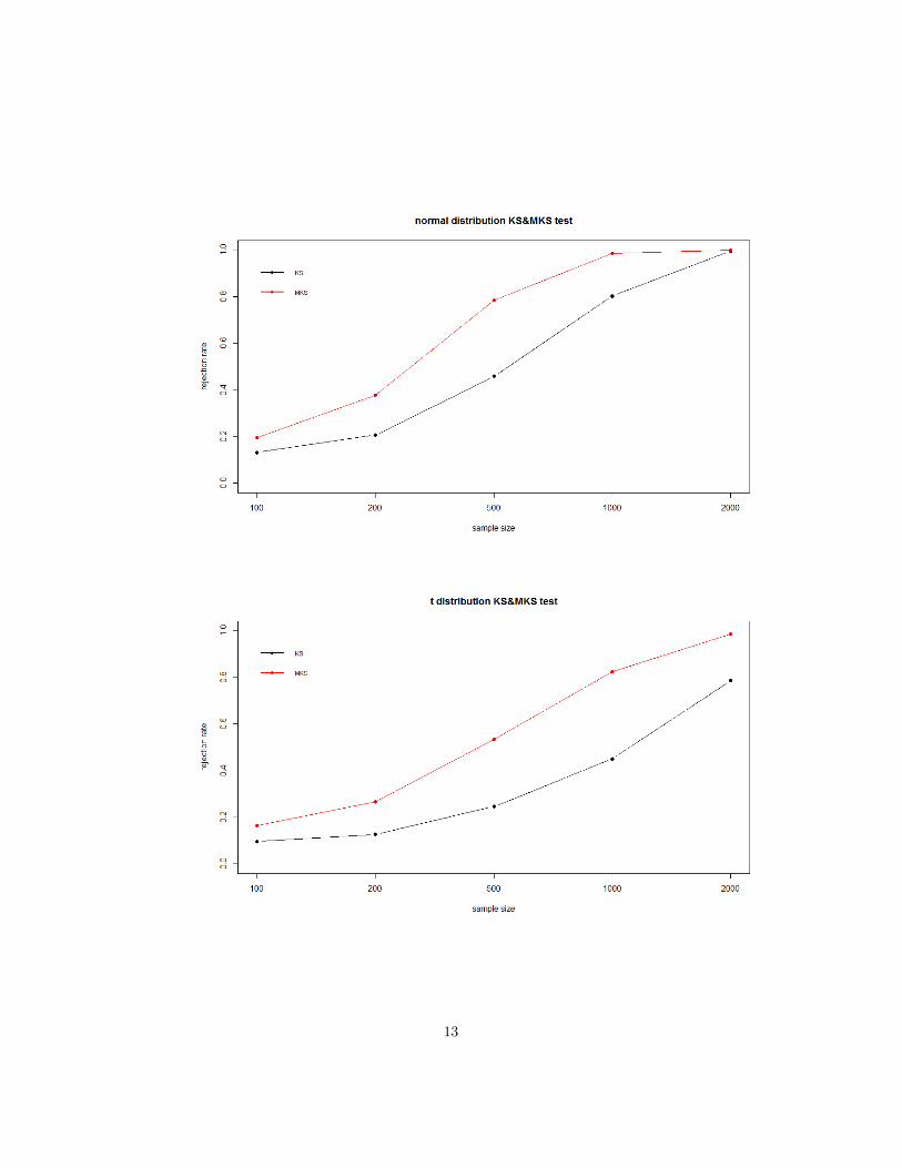
The next three plots are

12

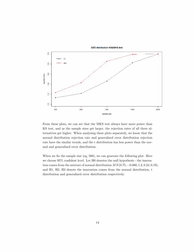
From these plots, we can see that the MKS test always have more power than

KS test, and as the sample sizes get larger, the rejection rates of all three al-

ternatives get higher. When analysing these plots separately, we know that the

normal distribution rejection rate and generalized error distribution rejection

rate have the similar trends, and the t distribution has less power than the nor-

mal and generalized error distribution.

When we fix the sample size (eg, 500), we can generate the following plot. Here

we choose 95% confident level. Let H0 denotes the null hypothesis - the innova-

tion comes from the mixture of normal distributionMN(0.75,−0.080, 1.2, 0.24, 0.19),

and H1, H2, H3 denote the innovation comes from the normal distribution, t

distribution and generalized error distribution respectively.

14

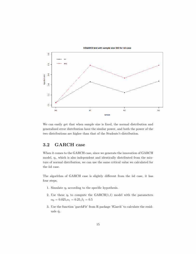
We can easily get that when sample size is fixed, the normal distribution and

generalized error distribution have the similar power, and both the power of the

two distributions are higher than that of the Students’t-distribution.

3.2 GARCH case

When it comes to the GARCH case, since we generate the innovation of GARCH

model, ηt, which is also independent and identically distributed from the mix-

ture of normal distribution, we can use the same critical value we calculated for

the iid case.

The algorithm of GARCH case is slightly different from the iid case, it has

four steps,

1. Simulate ηt according to the specific hypothesis.

2. Use these ηt to compute the GARCH(1,1) model with the parameters

α0 = 0.025,α1 = 0.25,β1 = 0.5

3. Use the function ’garchFit’ from R package ’fGarch’ to calculate the resid-

uals η̂t.

15

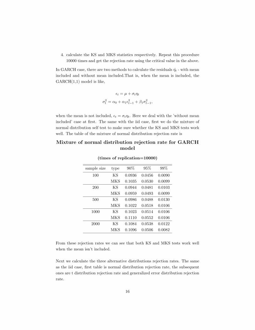
4. calculate the KS and MKS statistics respectively. Repeat this procedure

10000 times and get the rejection rate using the critical value in the above.

In GARCH case, there are two methods to calculate the residuals η̂t - with mean

included and without mean included.That is, when the mean is included, the

GARCH(1,1) model is like,

εt = µ+ σtηt

σ2t = α0 + α1ε

2t−1 + β1σ

2t−1,

when the mean is not included, εt = σtηt. Here we deal with the ’without mean

included’ case at first. The same with the iid case, first we do the mixture of

normal distribution self test to make sure whether the KS and MKS tests work

well. The table of the mixture of normal distribution rejection rate is

Mixture of normal distribution rejection rate for GARCHmodel



100 KS 0.0936 0.0456 0.0090

MKS 0.1035 0.0530 0.0099

200 KS 0.0944 0.0481 0.0103

MKS 0.0959 0.0493 0.0099

500 KS 0.0986 0.0488 0.0130

MKS 0.1022 0.0518 0.0106

1000 KS 0.1023 0.0514 0.0106

MKS 0.1110 0.0552 0.0106

2000 KS 0.1084 0.0538 0.0122

MKS 0.1096 0.0506 0.0082

From these rejection rates we can see that both KS and MKS tests work well

when the mean isn’t included.

Next we calculate the three alternative distributions rejection rates. The same

as the iid case, first table is normal distribution rejection rate, the subsequent

ones are t distribution rejection rate and generalized error distribution rejection

rate.

16

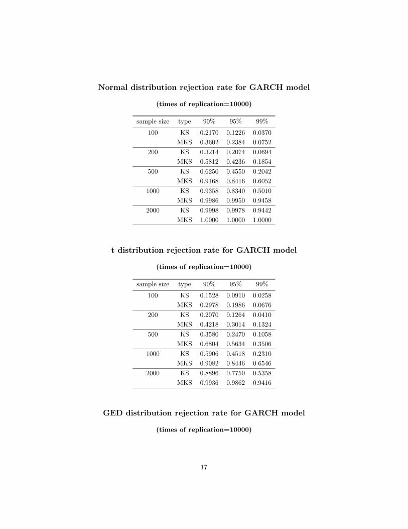
Normal distribution rejection rate for GARCH model



100 KS 0.2170 0.1226 0.0370

MKS 0.3602 0.2384 0.0752

200 KS 0.3214 0.2074 0.0694

MKS 0.5812 0.4236 0.1854

500 KS 0.6250 0.4550 0.2042

MKS 0.9168 0.8416 0.6052

1000 KS 0.9358 0.8340 0.5010

MKS 0.9986 0.9950 0.9458

2000 KS 0.9998 0.9978 0.9442

MKS 1.0000 1.0000 1.0000

t distribution rejection rate for GARCH model



100 KS 0.1528 0.0910 0.0258

MKS 0.2978 0.1986 0.0676

200 KS 0.2070 0.1264 0.0410

MKS 0.4218 0.3014 0.1324

500 KS 0.3580 0.2470 0.1058

MKS 0.6804 0.5634 0.3506

1000 KS 0.5906 0.4518 0.2310

MKS 0.9082 0.8446 0.6546

2000 KS 0.8896 0.7750 0.5358

MKS 0.9936 0.9862 0.9416

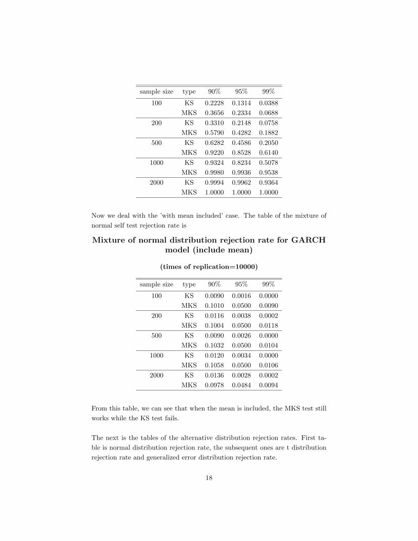
GED distribution rejection rate for GARCH model


17


100 KS 0.2228 0.1314 0.0388

MKS 0.3656 0.2334 0.0688

200 KS 0.3310 0.2148 0.0758

MKS 0.5790 0.4282 0.1882

500 KS 0.6282 0.4586 0.2050

MKS 0.9220 0.8528 0.6140

1000 KS 0.9324 0.8234 0.5078

MKS 0.9980 0.9936 0.9538

2000 KS 0.9994 0.9962 0.9364

MKS 1.0000 1.0000 1.0000

Now we deal with the ’with mean included’ case. The table of the mixture of

normal self test rejection rate is

Mixture of normal distribution rejection rate for GARCHmodel (include mean)



100 KS 0.0090 0.0016 0.0000

MKS 0.1010 0.0500 0.0090

200 KS 0.0116 0.0038 0.0002

MKS 0.1004 0.0500 0.0118

500 KS 0.0090 0.0026 0.0000

MKS 0.1032 0.0500 0.0104

1000 KS 0.0120 0.0034 0.0000

MKS 0.1058 0.0500 0.0106

2000 KS 0.0136 0.0028 0.0002

MKS 0.0978 0.0484 0.0094

From this table, we can see that when the mean is included, the MKS test still

works while the KS test fails.

The next is the tables of the alternative distribution rejection rates. First ta-

ble is normal distribution rejection rate, the subsequent ones are t distribution

rejection rate and generalized error distribution rejection rate.

18

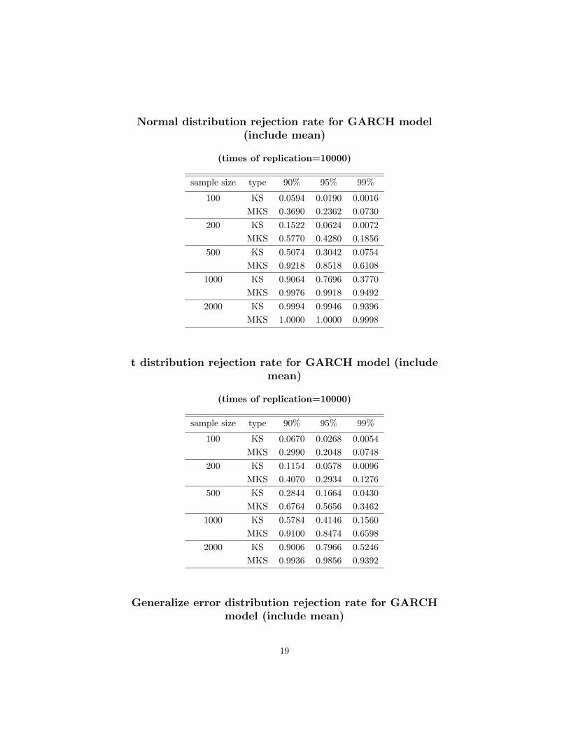
Normal distribution rejection rate for GARCH model(include mean)



100 KS 0.0594 0.0190 0.0016

MKS 0.3690 0.2362 0.0730

200 KS 0.1522 0.0624 0.0072

MKS 0.5770 0.4280 0.1856

500 KS 0.5074 0.3042 0.0754

MKS 0.9218 0.8518 0.6108

1000 KS 0.9064 0.7696 0.3770

MKS 0.9976 0.9918 0.9492

2000 KS 0.9994 0.9946 0.9396

MKS 1.0000 1.0000 0.9998

t distribution rejection rate for GARCH model (includemean)



100 KS 0.0670 0.0268 0.0054

MKS 0.2990 0.2048 0.0748

200 KS 0.1154 0.0578 0.0096

MKS 0.4070 0.2934 0.1276

500 KS 0.2844 0.1664 0.0430

MKS 0.6764 0.5656 0.3462

1000 KS 0.5784 0.4146 0.1560

MKS 0.9100 0.8474 0.6598

2000 KS 0.9006 0.7966 0.5246

MKS 0.9936 0.9856 0.9392

Generalize error distribution rejection rate for GARCHmodel (include mean)

19



100 KS 0.0670 0.0268 0.0054

MKS 0.2990 0.2048 0.0748

200 KS 0.1406 0.0614 0.0070

MKS 0.5684 0.4256 0.1796

500 KS 0.5048 0.3060 0.0820

MKS 0.9200 0.8466 0.6228

1000 KS 0.9130 0.7846 0.3964

MKS 0.9984 0.9924 0.9462

2000 KS 0.9998 0.9972 0.9374

MKS 1.0000 1.0000 0.9996

Based these tables, we can do some plots in order to make the outcomes more

observable.

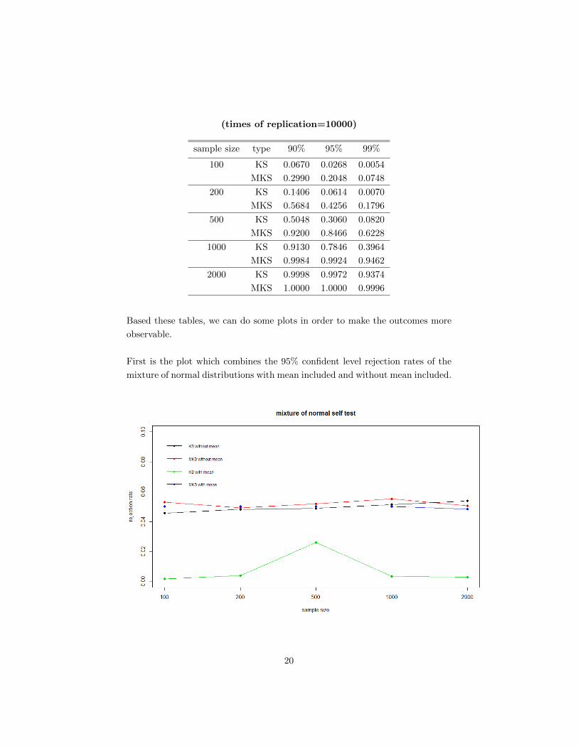
First is the plot which combines the 95% confident level rejection rates of the

mixture of normal distributions with mean included and without mean included.

20

From this plot we can easily see that when the mean is not included, both KS

and MKS tests work. But when the mean is included, the KS test fails and

MKS test still works.

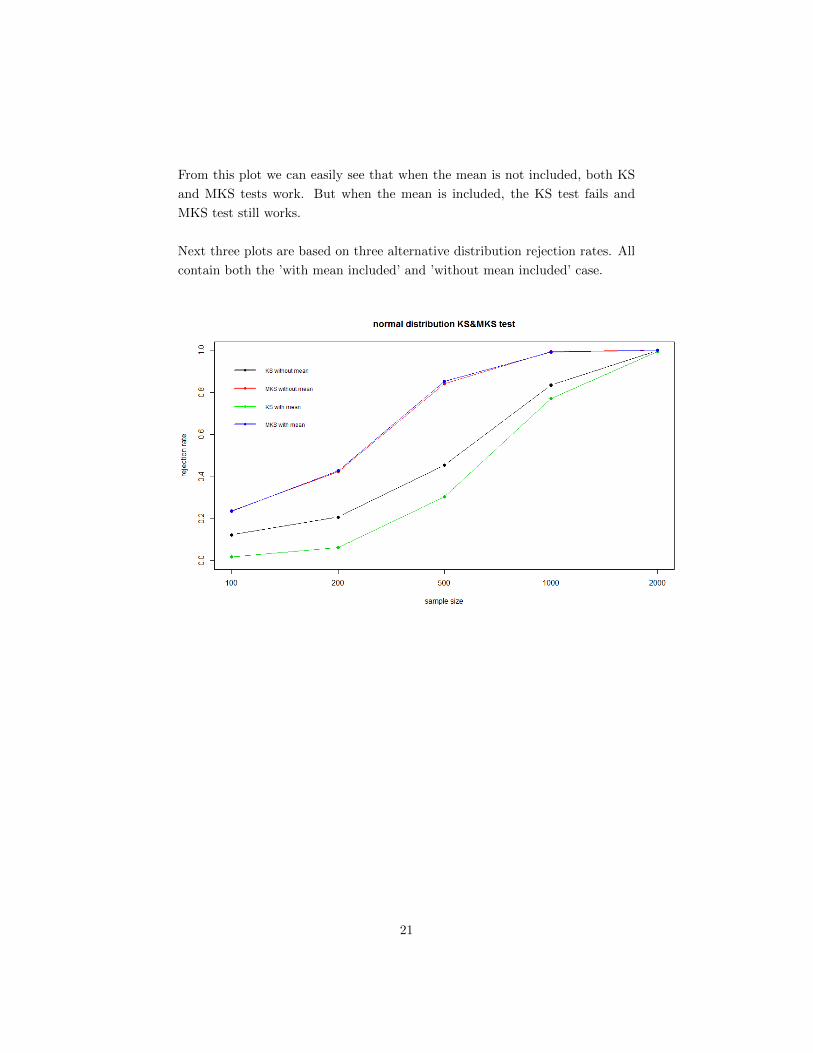
Next three plots are based on three alternative distribution rejection rates. All

contain both the ’with mean included’ and ’without mean included’ case.

21

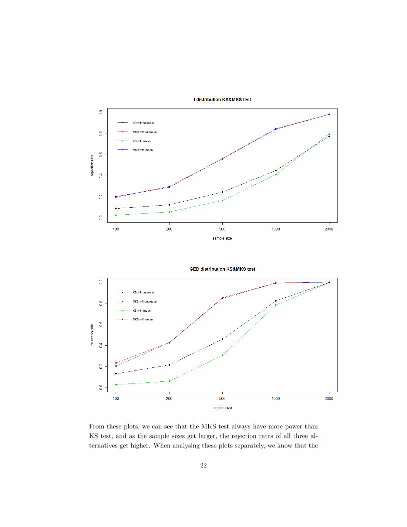
From these plots, we can see that the MKS test always have more power than

KS test, and as the sample sizes get larger, the rejection rates of all three al-

ternatives get higher. When analysing these plots separately, we know that the

22

normal distribution rejection rate and generalized error distribution rejection

rate have the similar trends, and the t distribution has less power than the nor-

mal and generalized error distribution.

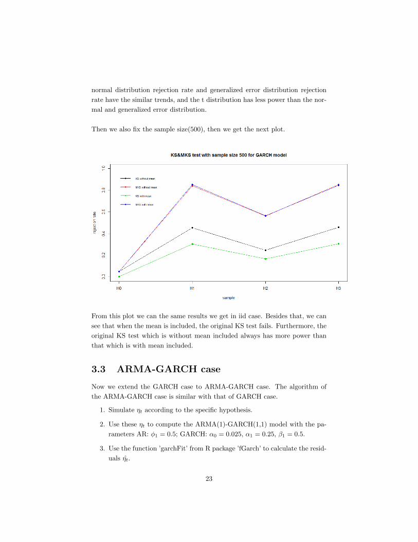
Then we also fix the sample size(500), then we get the next plot.

From this plot we can the same results we get in iid case. Besides that, we can

see that when the mean is included, the original KS test fails. Furthermore, the

original KS test which is without mean included always has more power than

that which is with mean included.

3.3 ARMA-GARCH case

Now we extend the GARCH case to ARMA-GARCH case. The algorithm of

the ARMA-GARCH case is similar with that of GARCH case.

1. Simulate ηt according to the specific hypothesis.

2. Use these ηt to compute the ARMA(1)-GARCH(1,1) model with the pa-

rameters AR: φ1 = 0.5; GARCH: α0 = 0.025, α1 = 0.25, β1 = 0.5.

3. Use the function ’garchFit’ from R package ’fGarch’ to calculate the resid-

uals η̂t.

23

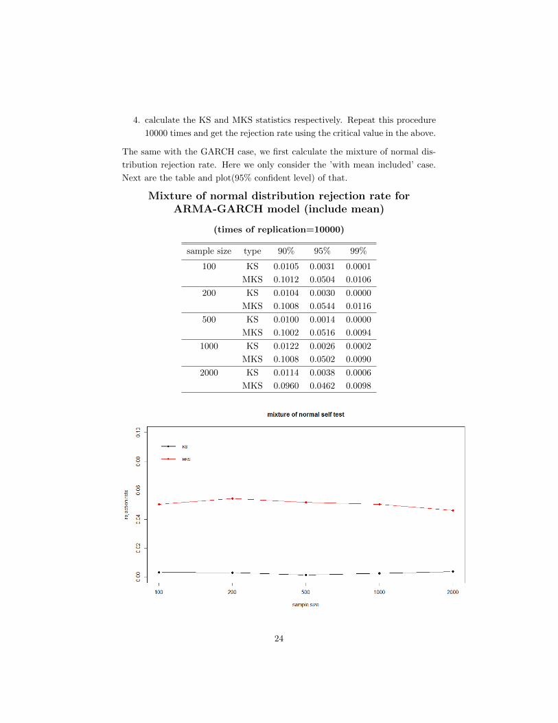
4. calculate the KS and MKS statistics respectively. Repeat this procedure

10000 times and get the rejection rate using the critical value in the above.

The same with the GARCH case, we first calculate the mixture of normal dis-

tribution rejection rate. Here we only consider the ’with mean included’ case.

Next are the table and plot(95% confident level) of that.

Mixture of normal distribution rejection rate forARMA-GARCH model (include mean)



100 KS 0.0105 0.0031 0.0001

MKS 0.1012 0.0504 0.0106

200 KS 0.0104 0.0030 0.0000

MKS 0.1008 0.0544 0.0116

500 KS 0.0100 0.0014 0.0000

MKS 0.1002 0.0516 0.0094

1000 KS 0.0122 0.0026 0.0002

MKS 0.1008 0.0502 0.0090

2000 KS 0.0114 0.0038 0.0006

MKS 0.0960 0.0462 0.0098

24

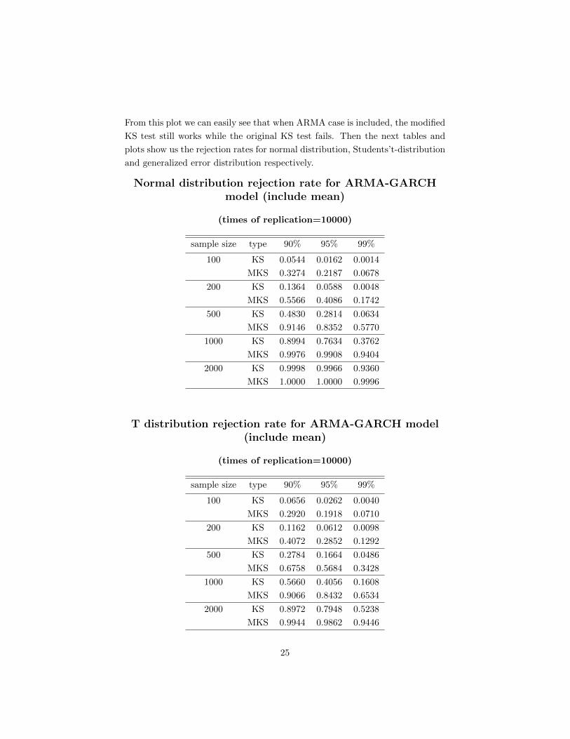
From this plot we can easily see that when ARMA case is included, the modified

KS test still works while the original KS test fails. Then the next tables and

plots show us the rejection rates for normal distribution, Students’t-distribution

and generalized error distribution respectively.

Normal distribution rejection rate for ARMA-GARCHmodel (include mean)



100 KS 0.0544 0.0162 0.0014

MKS 0.3274 0.2187 0.0678

200 KS 0.1364 0.0588 0.0048

MKS 0.5566 0.4086 0.1742

500 KS 0.4830 0.2814 0.0634

MKS 0.9146 0.8352 0.5770

1000 KS 0.8994 0.7634 0.3762

MKS 0.9976 0.9908 0.9404

2000 KS 0.9998 0.9966 0.9360

MKS 1.0000 1.0000 0.9996

T distribution rejection rate for ARMA-GARCH model(include mean)



100 KS 0.0656 0.0262 0.0040

MKS 0.2920 0.1918 0.0710

200 KS 0.1162 0.0612 0.0098

MKS 0.4072 0.2852 0.1292

500 KS 0.2784 0.1664 0.0486

MKS 0.6758 0.5684 0.3428

1000 KS 0.5660 0.4056 0.1608

MKS 0.9066 0.8432 0.6534

2000 KS 0.8972 0.7948 0.5238

MKS 0.9944 0.9862 0.9446

25

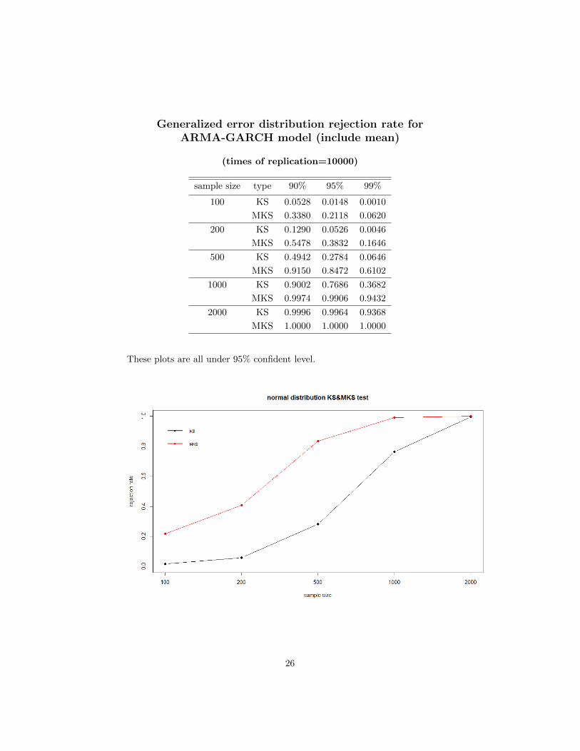
Generalized error distribution rejection rate forARMA-GARCH model (include mean)



100 KS 0.0528 0.0148 0.0010

MKS 0.3380 0.2118 0.0620

200 KS 0.1290 0.0526 0.0046

MKS 0.5478 0.3832 0.1646

500 KS 0.4942 0.2784 0.0646

MKS 0.9150 0.8472 0.6102

1000 KS 0.9002 0.7686 0.3682

MKS 0.9974 0.9906 0.9432

2000 KS 0.9996 0.9964 0.9368

MKS 1.0000 1.0000 1.0000

These plots are all under 95% confident level.

26

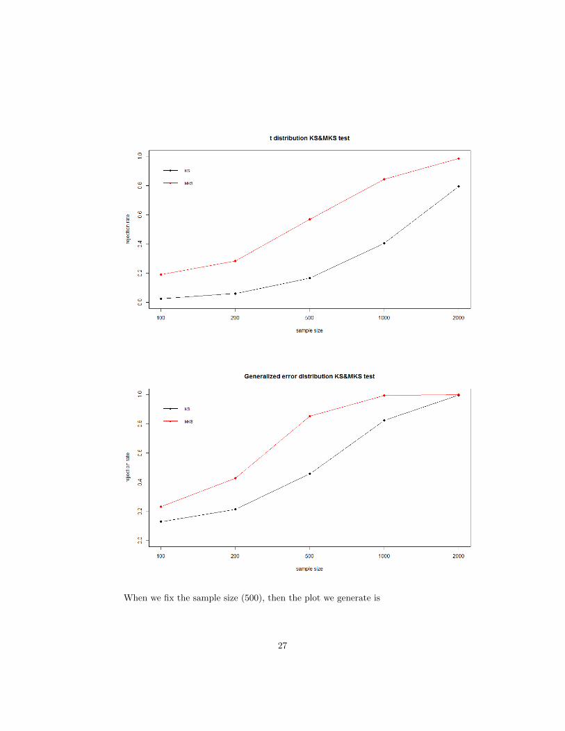
When we fix the sample size (500), then the plot we generate is

27

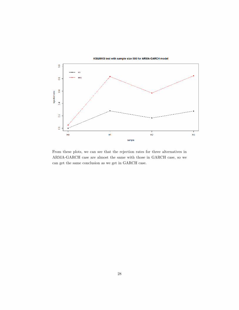
From these plots, we can see that the rejection rates for three alternatives in

ARMA-GARCH case are almost the same with those in GARCH case, so we

can get the same conclusion as we get in GARCH case.

28

Chapter 4

Conclusions and Future

work

In this project, we want to test whether the innovation of GARCH model comes

from the mixture of normal distribution MN ∼ (0.75,−0.08, 1.2, 0.24, 0.19),

which is the null hypothesis. Then we use KS test and modified KS test to

complete this objective. After getting the critical value, we can conduct the

simulation study for different sample sizes and three alternative distributions -

Normal distribution, Student’s t-distribution and Generalized error distribution

to calculate the rejection rate. Here are three main conclusions:

1. The original KS test fails when mean is included and has poor power under

the alternatives.

2. The modified KS test works regardless of whether the mean is included or

not and has relative high power under the alternatives

3. When sample size is fixed, the normal distribution and generalized er-

ror distribution have the similar power, and both the power of the two

distributions are higher than that of the Students’t-distribution.

All the results we mention before is based on the known parameters - the pa-

rameters of mixture of normal distribution are fixed and set up at first. But

for real data such as the return rate of a stock, we don’t know the parameters

when we fit the data in to a mixture of normal distribution. So further study is

needed in this regard.

29

Chapter 5

Acknowledgement

I would like the express the deepest appreciation to my supervisor - Dr. Hao

Yu. Without his patient help and guidance I couldn’t finish this project. It’s

also a pleasure for me to be under his supervision.

30

Bibliography

[1] R. Engle. Autoregressive conditional heteroscedasticity with estimates of the

variance of United Kingdom inflation. Econometrica 50:987 - 1007, 1982.

[2] T. Bollerslev. Generalized autoregressive conditional heteroskedasticity.

Journal of Econometrics 31:307 - 327,1986.

[3] J. Kawczak, R. Kulperger, and H. Yu. The empirical distribution function

and partial sum process of residuals from a stationary ARCH with drift

process. Ann. Inst. Statist. Math 57:747 - 765, 2005.

[4] H. Yu. Empirical processes of standardized residuals for a class of conditional

heteroscedasticmodels. Preprint

31

Dong Zhang's project

Documents

Transcript of Dong Zhang's project