1 Pertemuan 7 Variabel Acak-1 Matakuliah: A0064 / Statistik Ekonomi Tahun: 2005 Versi: 1/1.

1

Pertemuan 7Variabel Acak-1

Matakuliah : A0064 / Statistik Ekonomi

Tahun : 2005

Versi : 1/1

2

Learning Outcomes

Pada akhir pertemuan ini, diharapkan mahasiswa

akan mampu :

• Menghitung beberapa persoalan yang berkaitan dengan nilai harapan variabel acak diskrit, bernoulli, dan binomial

3

Outline Materi

• Nilai Harapan Variabel Acak Diskrit

• Variabel Acak Bernoulli

• Variabel Acak Binomial

COMPLETE 5 t h e d i t i o nBUSINESS STATISTICS

Aczel/SounderpandianMcGraw-Hill/Irwin © The McGraw-Hill Companies, Inc., 2002

3-4

Using Statistics Expected Values of Discrete Random

Variables The Binomial Distribution Other Discrete Probability Distributions Continuous Random Variables Using the Computer Summary and Review of Terms

Random Variables3



3-5

Consider the different possible orderings of boy (B) and girl (G) in four sequential births. There are 2*2*2*2=24 = 16 possibilities, so the sample space is:

BBBB BGBB GBBB GGBB BBBG BGBG GBBG GGBGBBGB BGGB GBGB GGGBBBGG BGGG GBGG GGGG

If girl and boy are each equally likely [P(G)=P(B) = 1/2], and the gender of each child is independent of that of the previous child, then the probability of each of these 16 possibilities is:(1/2)(1/2)(1/2)(1/2) = 1/16.

3-1 Using Statistics



3-6

Now count the number of girls in each set of four sequential births:

BBBB (0) BGBB (1) GBBB (1) GGBB (2)BBBG (1) BGBG (2) GBBG (2) GGBG (3)BBGB (1) BGGB (2) GBGB (2) GGGB (3)BBGG (2) BGGG (3) GBGG (3) GGGG (4)

Notice that:• each possible outcome is assigned a single numeric value,• all outcomes are assigned a numeric value, and• the value assigned varies over the outcomes.

The count of the number of girls is a random variable:

A random variable, X, is a function that assigns a single, but variable, value to each element of a sample space.

Random Variables



3-7

Random Variables (Continued)

BBBB BGBB GBBB

BBBG BBGB

GGBB GBBG BGBG

BGGB GBGB BBGG BGGG GBGG

GGGB GGBG

GGGG

0

1

2

3

4

XX

Sample SpaceSample Space

Points on the Points on the Real LineReal Line



3-8

Since the random variable X = 3 when any of the four outcomes BGGG, GBGG, GGBG, or GGGB occurs,

P(X = 3) = P(BGGG) + P(GBGG) + P(GGBG) + P(GGGB) = 4/16

The probability distribution of a random variable is a table that lists the possible values of the random variables and their associated probabilities.

x P(x)0 1/161 4/162 6/163 4/164 1/16 16/16=1

43210

0 .4

0 .3

0 .2

0 .1

N u m b e r o f g i r ls , x

P(x

)

0 .0 6 2 5

0 .2 5 0 0

0 .3 7 5 0

0 .2 5 0 0

0 .0 6 2 5

P ro b a b ility D is tr ib u tio n o f th e N u m b e r o f G ir ls in F o u r B ir th s

Random Variables (Continued)



3-9

Consider the experiment of tossing two six-sided dice. There are 36 possible outcomes. Let the random variable X represent the sum of the numbers on the two dice:

2 3 4 5 6 71,1 1,2 1,3 1,4 1,5 1,6 82,1 2,2 2,3 2,4 2,5 2,6 93,1 3,2 3,3 3,4 3,5 3,6 104,1 4,2 4,3 4,4 4,5 4,6 11

5,1 5,2 5,3 5,4 5,5 5,6 126,1 6,2 6,3 6,4 6,5 6,6

x P(x)*

2 1/363 2/364 3/365 4/366 5/367 6/368 5/369 4/3610 3/3611 2/3612 1/36

1

12111098765432

0.17

0.12

0.07

0.02

xp

(x)

Probability Distribution of Sum of Two Dice

* ( ) ( ( ) ) / Note that: P x x 6 7 362

Example 3-1



3-10

Probability of at least 1 switch: P(X 1) = 1 - P(0) = 1 - 0.1 = .9

Probability Distribution of the Number of Switches

x P(x)0 0.11 0.22 0.33 0.24 0.15 0.1

1

Probability of more than 2 switches: P(X > 2) = P(3) + P(4) + P(5) = 0.2 + 0.1 + 0.1 = 0.4

543210

0.4

0.3

0.2

0.1

0.0

x

P(x

)

The Probability Distribution of the Number of Switches

Example 3-2



3-11

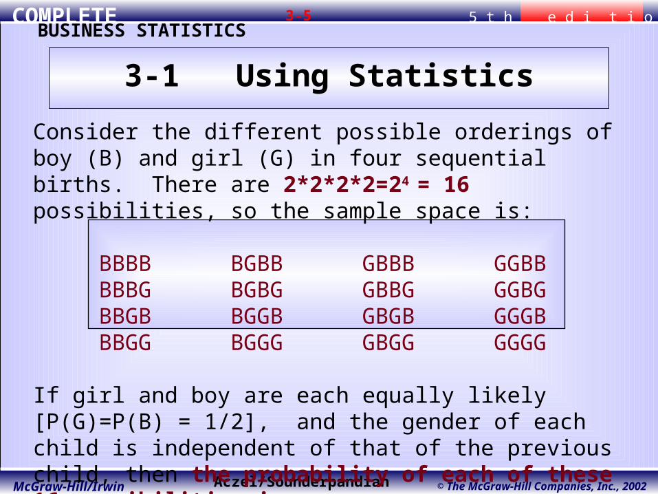
A discrete random variable: has a countable number of possible values has discrete jumps (or gaps) between successive values has measurable probability associated with individual values counts

A discrete random variable: has a countable number of possible values has discrete jumps (or gaps) between successive values has measurable probability associated with individual values counts

A continuous random variable: has an uncountably infinite number of possible values moves continuously from value to value has no measurable probability associated with each value measures (e.g.: height, weight, speed, value, duration, length)

A continuous random variable: has an uncountably infinite number of possible values moves continuously from value to value has no measurable probability associated with each value measures (e.g.: height, weight, speed, value, duration, length)

Discrete and Continuous Random Variables



3-12

1 0

1

0 1

. for all values of x.

2.

Corollary:

all x

P x

P x

P X

( )

( )

( )

The probability distribution of a discrete random variable X must satisfy the following two conditions.

Rules of Discrete Probability Distributions



3-13

F x P X x P iall i x

( ) ( ) ( )

The cumulative distribution function, F(x), of a discrete random variable X is:

x P(x) F(x)0 0.1 0.11 0.2 0.32 0.3 0.63 0.2 0.84 0.1 0.95 0.1 1.0

1 543210

1 .0

0 .9

0 .8

0 .7

0 .6

0 .5

0 .4

0 .3

0 .2

0 .1

0 .0

x

F(x

)

Cumulative Probability Distribution of the Number of Switches

Cumulative Distribution Function



3-14

x P(x) F(x)0 0.1 0.11 0.2 0.32 0.3 0.63 0.2 0.84 0.1 0.95 0.1 1.0

1

The probability that at most three switches will occur:

The Probability That at Most Three Switches W ill Occur

543210

0 .4

0 .3

0 .2

0 .1

0 .0

x

P(x

)

P X F( ) ( ) 3 3

Cumulative Distribution Function

Note:Note: P(X < 3) = F(3) = 0.8 = P(0) + P(1) + P(2) + P(3)



3-15

x P(x) F(x)0 0.1 0.11 0.2 0.32 0.3 0.63 0.2 0.84 0.1 0.95 0.1 1.0

1

The probability that more than one switch will occur:

543210

0 .4

0 .3

0 .2

0 .1

0 .0

x

P(x

)

P X F( ) ( ) 1 1 1

The Probability That More than One Switch Will Occur

F ( )1

Using Cumulative Probability Distributions (Figure 3-8)

Note:Note: P(X > 1) = P(X > 2) = 1 – P(X < 1) = 1 – F(1) = 1 – 0.3 = 0.7



3-16

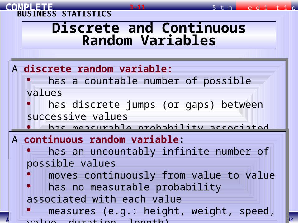
x P(x) F(x)0 0.1 0.11 0.2 0.32 0.3 0.63 0.2 0.84 0.1 0.95 0.1 1.0

1

The probability that anywhere from one to three switches will occur:

543210

0 .4

0 .3

0 .2

0 .1

0 .0

x

P(x

)

The Probability That Anywhere from One to Three Switches Will Occur

F ( )0

F ( )3

F X F F( ) ( ) ( )1 3 3 0

Using Cumulative Probability Distributions (Figure 3-9)

Note:Note: P(1 < X < 3) = P(X < 3) – P(X < 0) = F(3) – F(0) = 0.8 – 0.1 = 0.7



3-17

543210

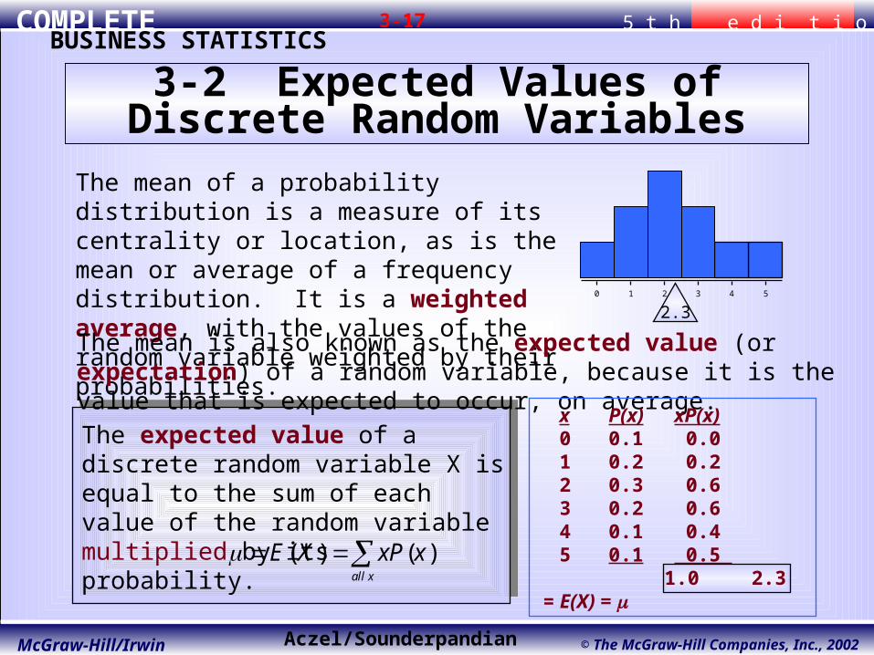
The mean of a probability distribution is a measure of its centrality or location, as is the mean or average of a frequency distribution. It is a weighted average, with the values of the random variable weighted by their probabilities.

The mean is also known as the expected value (or expectation) of a random variable, because it is the value that is expected to occur, on average.

The expected value of a discrete random variable X is equal to the sum of each value of the random variable multiplied by its probability.

E X xP xall x

( ) ( )

x P(x) xP(x)0 0.1 0.01 0.2 0.22 0.3 0.63 0.2 0.64 0.1 0.45 0.1 0.5 1.0 2.3 = E(X) =

2.3

3-2 Expected Values of Discrete Random Variables



3-18

Suppose you are playing a coin toss game in which you are paid $1 if the coin turns up heads and you lose $1 when the coin turns up tails. The expected value of this game is E(X) = 0. A game of chance with an expected payoff of 0 is called a fair game.

Suppose you are playing a coin toss game in which you are paid $1 if the coin turns up heads and you lose $1 when the coin turns up tails. The expected value of this game is E(X) = 0. A game of chance with an expected payoff of 0 is called a fair game.

x P(x) xP(x)-1 0.5 -0.50 1 0.5 0.50 1.0 0.00 =

E(X)=

-1 1 0

A Fair Game



3-19

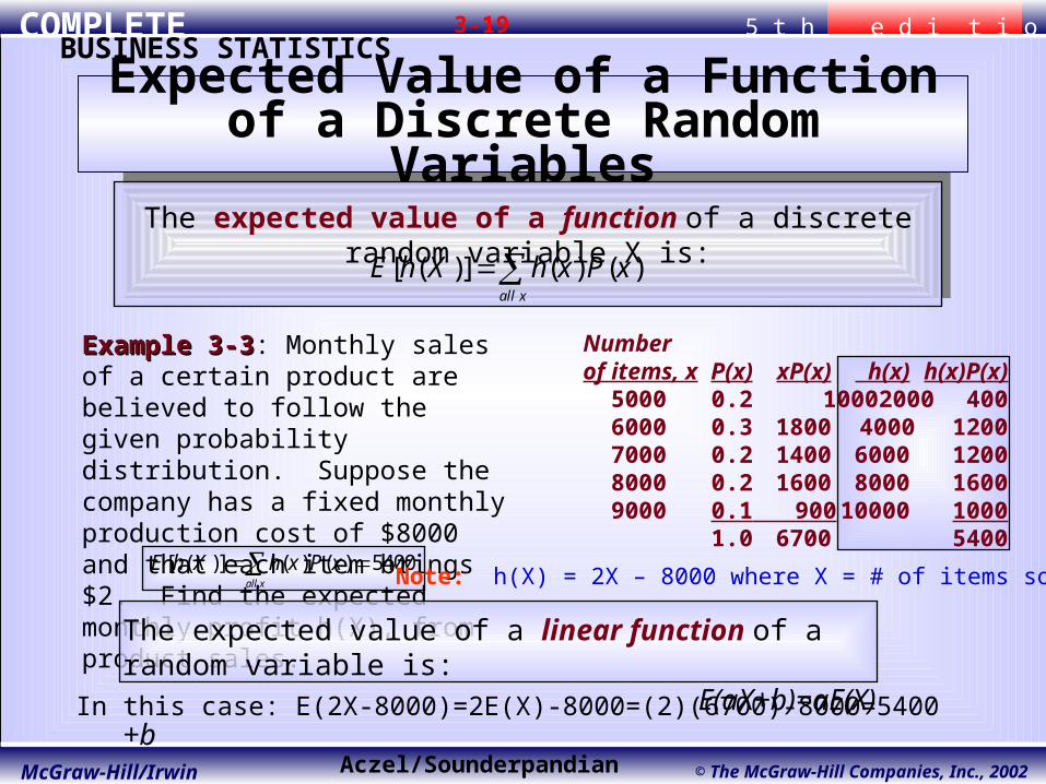
Number of items, x P(x) xP(x) h(x) h(x)P(x) 5000 0.2 1000 2000 400 6000 0.3 1800 4000 1200 7000 0.2 1400 6000 1200 8000 0.2 1600 8000 1600 9000 0.1 900 10000 1000

1.0 6700 5400

Example 3-3Example 3-3: Monthly sales of a certain product are believed to follow the given probability distribution. Suppose the company has a fixed monthly production cost of $8000 and that each item brings $2. Find the expected monthly profit h(X), from product sales.

E h X h x P xall x

[ ( )] ( ) ( ) 5400

The expected value of a function of a discrete random variable X is:

E h X h x P xall x

[ ( )] ( ) ( )

The expected value of a linear function of a random variable is: E(aX+b)=aE(X)+b

In this case: E(2X-8000)=2E(X)-8000=(2)(6700)-8000=5400

Expected Value of a Function of a Discrete Random Variables

Note: h(X) = 2X – 8000 where X = # of items sold



3-20

The variancevariance of a random variable is the expected squared deviation from the mean:

2 2 2

2 2 2

2

V X E X x P x

E X E X x P x xP x

all x

all x all x

( ) [( ) ] ( ) ( )

( ) [ ( )] ( ) ( )

The standard deviationstandard deviation of a random variable is the square root of its variance: SD X V X( ) ( )

Variance and Standard Deviation of a Random Variable



3-21

Number ofSwitches, x P(x) xP(x) (x-) (x-)2 P(x-)2 x2P(x)

0 0.1 0.0 -2.3 5.29 0.529 0.01 0.2 0.2 -1.3 1.69 0.338 0.22 0.3 0.6 -0.3 0.09 0.027 1.23 0.2 0.6 0.7 0.49 0.098 1.84 0.1 0.4 1.7 2.89 0.289 1.65 0.1 0.5 2.7 7.29 0.729 2.5

2.3 2.010 7.3

Number ofSwitches, x P(x) xP(x) (x-) (x-)2 P(x-)2 x2P(x)

0 0.1 0.0 -2.3 5.29 0.529 0.01 0.2 0.2 -1.3 1.69 0.338 0.22 0.3 0.6 -0.3 0.09 0.027 1.23 0.2 0.6 0.7 0.49 0.098 1.84 0.1 0.4 1.7 2.89 0.289 1.65 0.1 0.5 2.7 7.29 0.729 2.5

2.3 2.010 7.3

2 2

2 201

2 2

22

73 232 201

V X E X

xall x

P x

E X E X

xall x

P x xP xall x

( ) [( ) ]

( ) ( ) .

( ) [ ( )]

( ) ( )

. . .

Table 3-8

Variance and Standard Deviation of a Random Variable – using Example 3-2

Recall: = 2.3.



3-22

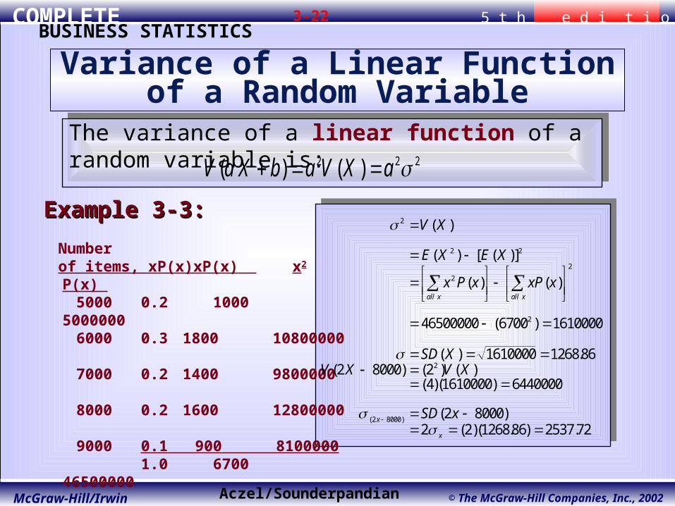
The variance of a linear function of a random variable is:

V a X b a V X a( ) ( ) 2 2 2

Number of items, x P(x) xP(x) x2 P(x) 5000 0.2 1000 5000000 6000 0.3 1800 10800000 7000 0.2 1400 9800000 8000 0.2 1600 12800000 9000 0.1 900 8100000

1.0 6700 46500000

Example 3-3:Example 3-3:

2

2 2

2

2

2

2

2 8000

46500000 6700 1610000

1610000 1268 862 8000 2

4 1610000 6440000

2 80002 2 1268 86 2537 72

V X

E X E X

x P x xP x

SD XV X V X

SD x

all x all x

x

x

( )

( ) [ ( )]

( ) ( )

( )

( ) .( ) ( ) ( )

( )( )

( )( )( . ) .

( )

Variance of a Linear Function of a Random Variable



3-23

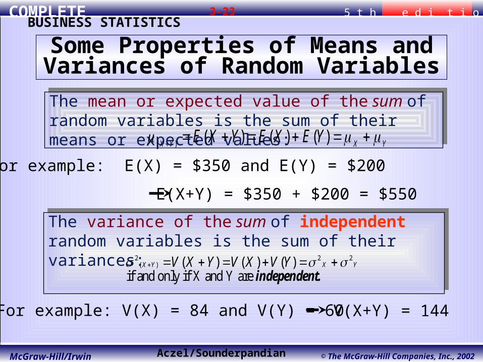
The mean or expected value of the sum of random variables is the sum of their means or expected values:

( ) ( ) ( ) ( )X Y X YE X Y E X E Y

For example: E(X) = $350 and E(Y) = $200

E(X+Y) = $350 + $200 = $550

The variance of the sum of independent random variables is the sum of their variances:

2 2 2( ) ( ) ( ) ( )X Y X YV X Y V X V Y

if and only if X and Y are independent.

For example: V(X) = 84 and V(Y) = 60 V(X+Y) = 144

Some Properties of Means and Variances of Random Variables



3-24

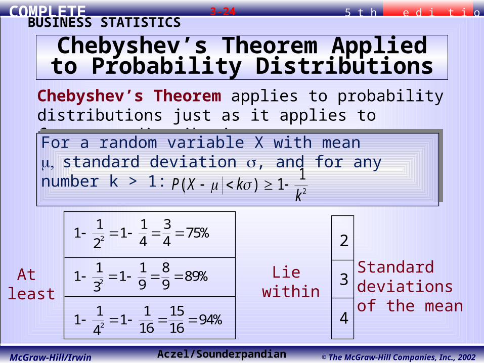
Chebyshev’s Theorem applies to probability distributions just as it applies to frequency distributions.

For a random variable X with mean standard deviation , and for any number k > 1:

P X kk

( ) 11

2

11

21

14

34

75%

11

31

19

89

89%

11

41

116

1516

94%

2

2

2

At least

Lie within

Standarddeviationsof the mean

2

3

4

Chebyshev’s Theorem Applied to Probability Distributions



3-25

Using the Template to Calculate statistics of h(x)



3-26

• If an experiment consists of a single trial and the outcome of the trial can only be either a success* or a failure, then the trial is called a Bernoulli trial.

• The number of success X in one Bernoulli trial, which can be 1 or 0, is a Bernoulli random variable.

• Note: If p is the probability of success in a Bernoulli experiment, the E(X) = p and V(X) = p(1 – p).

* The terms success and failure are simply statistical terms, and do not have positive or negative implications. In a production setting, finding a defective product may be termed a “success,” although it is not a positive result.

3-3 Bernoulli Random Variable



3-27

Consider a Bernoulli Process in which we have a sequence of n identical trials satisfying the following conditions:

1. Each trial has two possible outcomes, called success *and failure. The two outcomes are mutually exclusive and exhaustive.

2. The probability of success, denoted by p, remains constant from trial to trial. The probability of failure is denoted by q, where q = 1-p.

3. The n trials are independent. That is, the outcome of any trial does not affect the outcomes of the other trials.

A random variable, X, that counts the number of successes in n Bernoulli trials, where p is the probability of success* in any given trial, is said to follow the binomial probability distribution with parameters n (number of trials) and p (probability of success). We call X the binomial random variable.

* The terms success and failure are simply statistical terms, and do not have positive or negative implications. In a production setting, finding a defective product may be termed a “success,” although it is not a positive result.

The Binomial Random Variable



3-28

Suppose we toss a single fair and balanced coin five times in succession, and let X represent the number of heads.

There are 25 = 32 possible sequences of H and T (S and F) in the sample space for this experiment. Of these, there are 10 in which there are exactly 2 heads (X=2):

HHTTT HTHTH HTTHT HTTTH THHTT THTHT THTTH TTHHT TTHTH TTTHH

The probability of each of these 10 outcomes is p3q3 = (1/2)3(1/2)2=(1/32), so the probability of 2 heads in 5 tosses of a fair and balanced coin is:

P(X = 2) = 10 * (1/32) = (10/32) = .3125

10 (1/32)

Number of outcomeswith 2 heads

Probability of eachoutcome with 2 heads

Binomial Probabilities (Introduction)



3-29

10 (1/32)

Number of outcomeswith 2 heads

Probability of eachoutcome with 2 heads

P(X=2) = 10 * (1/32) = (10/32) = .3125Notice that this probability has two parts:

In general:

1. The probability of a given sequence of x successes out of n trials with probability of success p and probability of failure q is equal to:

pxq(n-x) nCxn

x

nx n x

!

!( )!

2. The number of different sequences of n trials that result in exactly x successes is equal to the number of choices of x elements out of a total of n elements. This number is denoted:

Binomial Probabilities (continued)



3-30

Number of successes, x Probability P(x)

0

1

2

3

n

1.00

nn

p q

nn

p q

nn

p q

nn

p q

nn n n

p q

n

n

n

n

n n n

!!( )!

!!( )!

!!( )!

!!( )!

!!( )!

( )

( )

( )

( )

( )

0 0

1 1

2 2

3 3

0 0

1 1

2 2

3 3

The binomial probability distribution:

where :p is the probability of success in a single trial,q = 1-p,n is the number of trials, andx is the number of successes.

P xn

xp q

nx n x

p qx n x x n x( )!

!( )!( ) ( )

The Binomial Probability Distribution



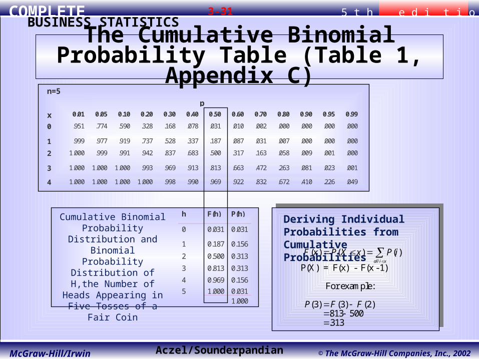
3-31

n=5

p

x 0.01 0.05 0.10 0.20 0.30 0.40 0.50 0.60 0.70 0.80 0.90 0.95 0.99

0 .951 .774 .590 .328 .168 .078 .031 .010 .002 .000 .000 .000 .000

1 .999 .977 .919 .737 .528 .337 .187 .087 .031 .007 .000 .000 .000

2 1.000 .999 .991 .942 .837 .683 .500 .317 .163 .058 .009 .001 .000

3 1.000 1.000 1.000 .993 .969 .913 .813 .663 .472 .263 .081 .023 .001

4 1.000 1.000 1.000 1.000 .998 .990 .969 .922 .832 .672 .410 .226 .049

h F(h) P(h)

0 0.031 0.031

1 0.187 0.156

2 0.500 0.313

3 0.813 0.313

4 0.969 0.156

5 1.000 0.0311.000

Cumulative Binomial Probability Distribution and

Binomial Probability Distribution of H,the

Number of Heads Appearing in Five Tosses of

a Fair Coin

F x P X x P i

P F F

all i x

( ) ( ) ( )

( ) ( ) ( ). ..

P(X) = F(x) - F(x - 1)

For example:

3 3 2813 500313

Deriving Individual Probabilities from Cumulative Probabilities

The Cumulative Binomial Probability Table (Table 1, Appendix C)



3-32

F x P X x P i

F P X

all i x

( ) ( ) ( )

( ) ( ) .

3 3 002

n=15p

.50 .60 .700 .000 .000 .0001 .000 .000 .0002 .004 .000 .0003 .018 .002 .0004 .059 .009 .001

... ... ... ...

60% of Brooke shares are owned by LeBow. A random sample of 15 shares is chosen. What is the probability that at most three of them will be found to be owned by LeBow?

Calculating Binomial Probabilities - Example



3-33

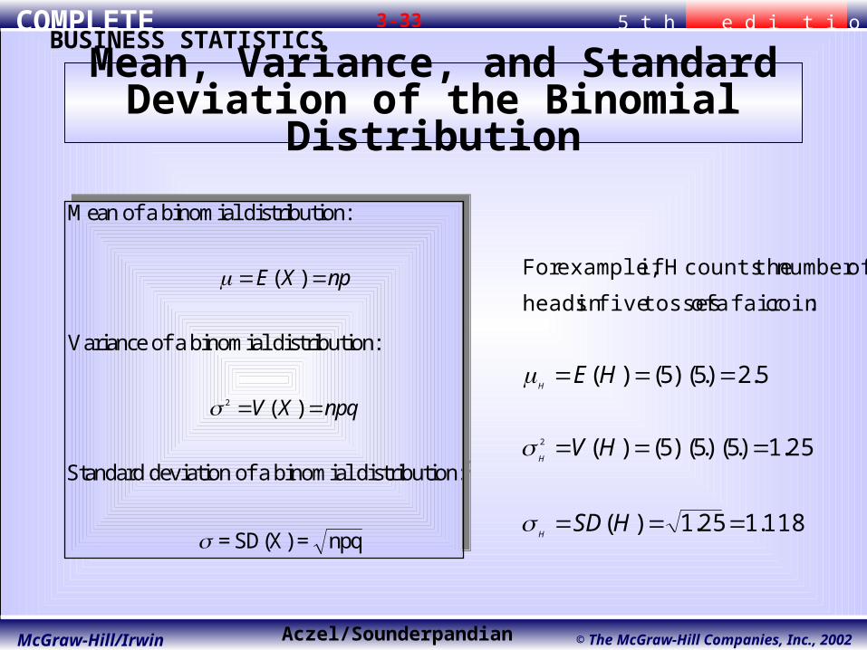
Mean of a binomial distribution:

Variance of a binomial distribution:

Standard deviation of a binomial distribution:

= SD(X) = npq

2

E X np

V X npq

( )

( )

Mean of a binomial distribution:

Variance of a binomial distribution:

Standard deviation of a binomial distribution:

= SD(X) = npq

2

E X np

V X npq

( )

( )

118.125.1)(

25.1)5)(.5)(.5()(

5.2)5)(.5()(

2

:coinfair a of tossesfivein heads

ofnumber thecounts H if example,For

HSD

HV

HE

H

H

H

Mean, Variance, and Standard Deviation of the Binomial Distribution



3-34

Calculating Binomial Probabilities using the Template



3-35

43210

0.7

0.6

0.5

0.4

0.3

0.2

0.1

0.0

x

P(x

)

Binomial Probability: n=4 p=0.5

43210

0.7

0.6

0.5

0.4

0.3

0.2

0.1

0.0

x

P(x

)


43210

0.7

0.6

0.5

0.4

0.3

0.2

0.1

0.0

x

P(x

)


109876543210

0.5

0.4

0.3

0.2

0.1

0.0

x

P(x

)


109876543210

0.5

0.4

0.3

0.2

0.1

0.0

x

P(x

)


109876543210

0.5

0.4

0.3

0.2

0.1

0.0

x

P(x

)


20191817161514131211109876543210

0.2

0.1

0.0

x

P(x

)


20191817161514131211109876543210

0.2

0.1

0.0

x

P(x

)


20191817161514131211109876543210

0.2

0.1

0.0

x

P(x

)


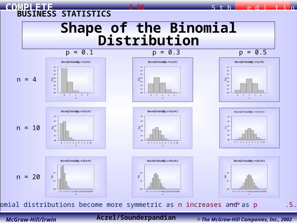
Binomial distributions become more symmetric as n increases and as p .5.

p = 0.1 p = 0.3 p = 0.5

n = 4

n = 10

n = 20

Shape of the Binomial Distribution



3-36

The negative binomial distribution is useful for determining the probability of the number of trials made until the desired number of successes are achieved in a sequence of Bernoulli trials. It counts the number of trials X to achieve the number of successes s with p being the probability of success on each trial.

The negative binomial distribution is useful for determining the probability of the number of trials made until the desired number of successes are achieved in a sequence of Bernoulli trials. It counts the number of trials X to achieve the number of successes s with p being the probability of success on each trial.

)()1(

1

1)(

sxp

sp

s

xxXP

:onDistributi Binomial Negative

2)1(2

:is varianceThe

:ismean The

p

ps

ps

3-5 Negative Binomial Distribution



3-37

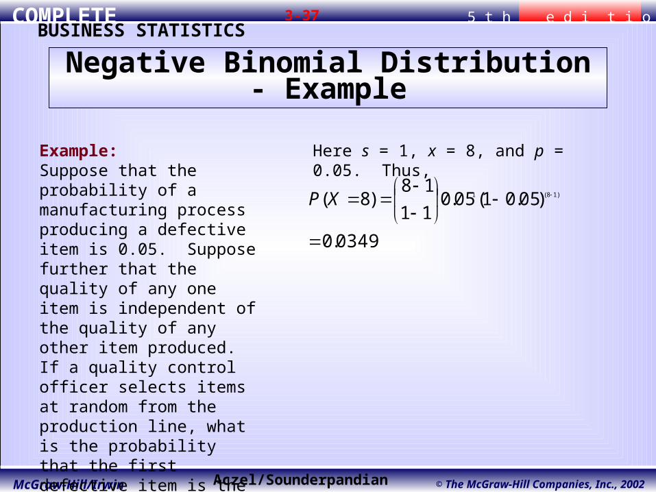
Negative Binomial Distribution - Example

Example:Suppose that the probability of a manufacturing process producing a defective item is 0.05. Suppose further that the quality of any one item is independent of the quality of any other item produced. If a quality control officer selects items at random from the production line, what is the probability that the first defective item is the eight item selected.

Here s = 1, x = 8, and p = 0.05. Thus,

0349.0

)05.01(05.011

18)8( )18(1

XP



3-38

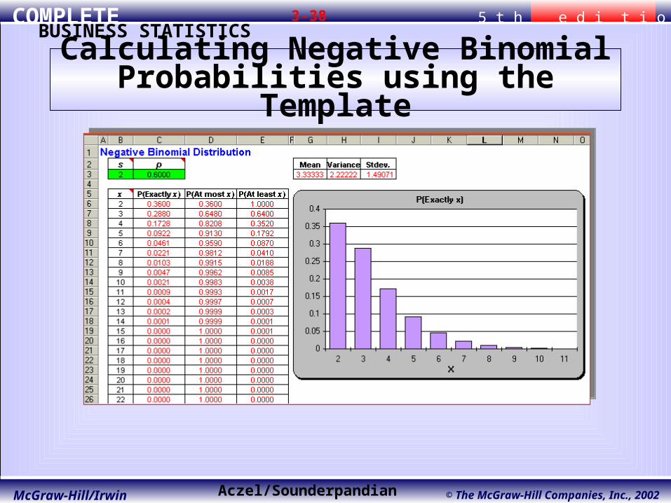
Calculating Negative Binomial Probabilities using the Template

39

Penutup

• Pembahasan dilanjutkan dengan materi Pokok-8 (Variabel Acak-2)

1 Pertemuan 7 Variabel Acak-1 Matakuliah: A0064 / Statistik Ekonomi Tahun: 2005 Versi: 1/1.

Documents

Transcript of 1 Pertemuan 7 Variabel Acak-1 Matakuliah: A0064 / Statistik Ekonomi Tahun: 2005 Versi: 1/1.